Chapter 1 Introduction to R
1.1 Getting help
You can find R on the official web site http://www.r-project.org/. It is available for Windows, Mac and Linux. As for any open source software, there are several manuals on R that can be downloaded from the internet for free. On the web site \href{http://cran.r-project.org/manuals.html, you will find detailed manuals for both users and developers. I recommend going through sections 1 to 9 of “An Introduction to R”, which will give you what you need to get started. The manual “R Data Import/Export” is a complete reference on how to deal with data from different sources (Stata, Matlab, Excel, etc.). There are also manuals specialized in econometrics. I suggest downloading http://cran.r-project.org/doc/contrib/Farnsworth-EconometricsInR.pdf. Finally, there are several books published by Springer for any area of econometrics which are not too expensive.
There are also tools integrated in R which are helpful when we are looking for a particular function or when we want to know how to use it. Suppose we want to know how to generate random numbers, but we don’t know the name of the function. We can search using key words:
which gives a list of functions for which “Normal Distribution” is in the description. For example, one of the results is “stats::Normal The Normal Distribution”, which means that the function “Normal” can be found in the package “stats”. The latter is included in R and therefore do not need to be added. However, the result “mnormt::dmnorm Multivariate normal distribution” refers to the function dmnorm which belongs to the package mvtnorm of Genz et al. (2011). This is one of the many packages that can be found on CRAN (see the list here: http://probability.ca/cran/web/packages/ and which can be installed using:
Once we have found the function we are looking for, we use the help function in order to learn the syntax. For example, if we are interested by the above result “Normal”, we type:
Notice that R is case sensitive. If you type help("normal"), you will get an error message. There are four functions associated with the term “Normal”. The help file starts with the syntax of these functions:
dnorm(x, mean = 0, sd = 1, log = FALSE)
pnorm(q, mean = 0, sd = 1, lower.tail = TRUE, log.p = FALSE)
qnorm(p, mean = 0, sd = 1, lower.tail = TRUE, log.p = FALSE)
rnorm(n, mean = 0, sd = 1)
Some arguments such as mean have default values and others such as x or q require a value. Here is some examples:
- The density of a N(0,1) evaluated at 0.5:
## [1] 0.3520653- The logarithm of the density of a N(0,1) evaluated at 0.5:
## [1] -1.043939- The density of a N(5,10) evaluated at 2:
## [1] 0.08044102- 5 pseudo random numbers from a N(0,1) using the seed 123:
## [1] -0.56047565 -0.23017749 1.55870831 0.07050839 0.12928774There are no secret tricks to learn a computer language. You need to sit down and work hard. The best way is to think about a numerical project and try to do it. And remember that if you have a problem, someone must have gone through the same. The answer is probably somewhere in a newsgroup. Internet search engines such as http://Google.ca are therefore endless sources of information. You can even participate and ask a question. But remember that the persons who answer are usually very friendly and work for free. Therefore, show them that you have made an effort before asking a question otherwise you could get the answer rtfm (read the f… manual).
Exercise 1.1 (Using help) Using the help or help.search, try to find a function that: (i) solves the system \(Ax=b\), (ii) estimates a linear model by OLS, (iii) gives you the number of characters in a string such as “hello” and (iv) computes the mean of each column of a matrix.
1.2 The basic concepts
1.2.1 Understanding the structure
R is an object-oriented language. The only difference between an object-oriented language and one which is not object-oriented is the organization of functions and elements. For example, the following
## [1] 1means that the new object x receives all the attributes of the right-hand side. In that case, the operators = and <- are identical. However, it is often suggested to always use the latter when defining an object. The former is used when we set the options in a function:
##      [,1]
## [1,]    1
To see the difference, the two-line code above can be written in one single line as:
##      [,1]
## [1,]    1
It defines the object y and then print it. In that case, the operator = cannot be used; try
An object is defined by its attributes and classes. Objects of some classes don’t have any attributes and some have many. For example, \(x\) and \(y\), defined above, look identical. But they are different objects. We can obtain the classes associated with an object by using the function is:
## [1] "numeric" "vector"## [1] "matrix" "array" "structure" "vector"and the attributes with attributes:
## NULL## $dim
## [1] 1 1The difference between these two objects is that \(x\) does not have the attribute dim which gives the dimension of an array. Therefore we could make \(x\) identical to \(y\) simply by adding the attribute dim to it as follows:
## [1] "matrix" "array" "structure" "vector"However, this is not the most efficient way to transform the object \(x\). We would obtain the same result with the command x <- as.matrix(x). It is very important to understand the difference between vectors with and without the attribute dim. The usual matrix operations can be performed only if the objects have the attribute dim. If they don’t, the operations can produce unexpected results. To see that, let \(A\) be a \(2\times 2\) matrix and \(x\) be a simple vector (without dim) containing two elements.
##      [,1] [,2]
## [1,]    1    3
## [2,] 2 4## [1] 1 2Additions of two matrices are allowed only if the dimensions coincide. Because \(x\) does not have any dimension, the operation \(A+x\) is allowed. But we have to be careful with how R treats such operations. In fact, a matrix of the same dimension as \(A\) is constructed by repeating the vector \(x\) until the total number of elements is equal to the number of elements of \(A\). Therefore, the number of elements of \(A\) should be a multiple of the number of elements of \(x\). A warning message is printed otherwise (try to experiment as much cases as possible to make sure you understand). The result is:
##      [,1] [,2]
## [1,]    2    4
## [2,]    4    6
However, if \(x\) is a \(2\times 1\) matrix, R returns an error message (Here I use the function try which returns the result if the operation is allowed and an error message otherwise):
## Error in x + A : non-conformable arrays## [1] "Error in x + A : non-conformable arrays\n"This way of treating operations may seem confusing at first, but it happens to be very useful in some cases. Suppose you have a \(T\times N\) matrix \(R\) of asset returns. Each column represents a different time series of returns. You also have a time series of returns on the three-month US treasury bill (\(R_f\)) that you want to use as proxy for the risk-free rate. To compute a time series of excess returns of each asset (\(Z_{it}=R_{it}-R_{ft}\)), you can simply define the vector of risk-free rates as a simple vector and do
There are also different kinds of vector. We can create a vector of messages:
## [1] "character"           "vector"              "data.frameRowLabels"
## [4] "SuperClassMethod"
It is a vector, which means that it is a collection of elements, but we don’t see the class “numeric”. Therefore, mathematical operations are not allowed on that kind of objects. In C++, which is probably the most popular object-oriented language for software developers, you can redefine the operator “+” for vectors of characters. It would, for example, construct a new vector by combining the characters of each vector. The operator “+” would react differently whether the vector is numeric or not. There is no point of having such operators in R, but it shows how it works. Many functions are built in such a way that they react differently depending on the type of objects. We call them “methods”. A method is a function that adapts itself to the class of the object. An example of method is summary. We can see the type of objects that this method deals with:
##  [1] summary.aov                         summary.aovlist*
##  [3] summary.aspell*                     summary.check_packages_in_dir*
##  [5] summary.connection                  summary.data.frame
##  [7] summary.Date                        summary.default
##  [9] summary.difftime                    summary.ecdf*
## [11] summary.factor                      summary.free1way*
## [13] summary.glm                         summary.infl*
## [15] summary.lm                          summary.loess*
## [17] summary.manova                      summary.matrix
## [19] summary.mlm*                        summary.nls*
## [21] summary.packageStatus*              summary.POSIXct
## [23] summary.POSIXlt                     summary.ppr*
## [25] summary.prcomp*                     summary.princomp*
## [27] summary.proc_time                   summary.rlang_error*
## [29] summary.rlang_message*              summary.rlang_trace*
## [31] summary.rlang_warning*              summary.rlang:::list_of_conditions*
## [33] summary.srcfile                     summary.srcref
## [35] summary.stepfun                     summary.stl*
## [37] summary.table                       summary.tukeysmooth*
## [39] summary.warnings
## see '?methods' for accessing help and source code
The class of the object appears after the dot. So, summary will treat objects of class “matrix” differently from objects of class, say, “data.frame”. Other classes not listed are treated by summary.default. For example, let \(X\) be a data.frame, than summary produces:
## Warning in matrix(runif(24), 4, 3): data length differs from size of matrix:
## [24 != 4 x 3]## Consumption Income Wealth
## Min. :0.2876 Min. :0.04556 Min. :0.4533
## 1st Qu.:0.3786 1st Qu.:0.40747 1st Qu.:0.4558
## Median :0.5986 Median :0.71026 Median :0.5040
## Mean :0.5920 Mean :0.60164 Mean :0.6046
## 3rd Qu.:0.8120 3rd Qu.:0.90443 3rd Qu.:0.6528
## Max. :0.8830 Max. :0.94047 Max. :0.9568If we create an object of class “lm” which is create by the OLS procedure lm, the summary method produces very different results:
##
## Call:
## lm(formula = Income ~ Consumption, data = X)
##
## Residuals:
##       1       2       3       4
##  0.1994 -0.4662 -0.1573  0.4241
##
## Coefficients:
##             Estimate Std. Error t value Pr(>|t|)
## (Intercept)   0.8728     0.6181   1.412    0.293
## Consumption  -0.4580     0.9621  -0.476    0.681
##
## Residual standard error: 0.4805 on 2 degrees of freedom
## Multiple R-squared:  0.1018, Adjusted R-squared:  -0.3473
## F-statistic: 0.2266 on 1 and 2 DF,  p-value: 0.681
In fact, every function produces an object of some kind. Even summary does:
## [1] "table" "oldClass"It is very useful because you can store all your results in different variables and save it in a file. For Example, if we estimate two models and want to save the properties of the data only, we would proceed this way:
res1 <-   lm(Income~Consumption,data=X)
res2 <- lm(Wealth~Consumption,data=X)
sum_stat <- summary(X)
save(res1,res2,sum_stat,file="data/all_result.rda")
rm(list=ls())
(the last line deletes all objects from the workspace) Then, you can reload later and analyze the results:
## Analysis of Variance Table
##
## Response: Income
##             Df  Sum Sq  Mean Sq F value Pr(>F)
## Consumption  1 0.05232 0.052319  0.2266  0.681
## Residuals    2 0.46167 0.230837
There are two categories of classes: S3 and S4. Functions that produce S3/class objects, like lm, are lists of elements. An element of a list can be extracted using $. You can obtain the names of each element with the names. For example, objects produced by lm contain the following elements:
##  [1] "coefficients"  "residuals"     "effects"       "rank"
##  [5] "fitted.values" "assign"        "qr"            "df.residual"
##  [9] "xlevels"       "call"          "terms"         "model"
If there is no conflict with other elements, you can only use the first letters:
## (Intercept) Consumption
## 0.8727695 -0.4580178## (Intercept) Consumption
## 0.8727695 -0.4580178## (Intercept) Consumption
## 0.8727695 -0.4580178For S4/class objects, the elements are called slots which may themself be S3/class objects. The unit root test procedure adfTest from the package “fUnitRoots” of Wuertz, others, and SOURCE file (2009) is an example of functions producing S4/class objects. Let us first create it:
## Warning in adfTest(x, lags = 2, type = "ct"): p-value smaller than printed
## p-value
The elements of S4/class objects can be extracted using @. We can obtain the names of the slots as follows:
## [1] "call" "data" "test" "title" "description"The slot “test” is a list as we can see:
## [1] "data.name" "statistic" "p.value" "parameter" "lm"Some elements are just values, as for “statistic” and “p.value”:
## Dickey-Fuller
## -7.904307##
## 0.01Others are S3/class objects like “lm” which contains the results of the OLS estimation:
##
## Call:
## lm(formula = y.diff ~ y.lag.1 + 1 + tt + y.diff.lag)
##
## Residuals:
##      Min       1Q   Median       3Q      Max
## -2.25260 -0.65132 -0.08469  0.62403  2.96349
##
## Coefficients:
##               Estimate Std. Error t value Pr(>|t|)
## (Intercept) -0.0150866  0.1382080  -0.109    0.913
## y.lag.1     -1.0628340  0.1344626  -7.904 2.05e-13 ***
## tt           0.0001167  0.0011923   0.098    0.922
## y.diff.lag1 -0.0097415  0.1055491  -0.092    0.927
## y.diff.lag2 -0.0921900  0.0717865  -1.284    0.201
## ---
## Signif. codes:  0 '***' 0.001 '**' 0.01 '*' 0.05 '.' 0.1 ' ' 1
##
## Residual standard error: 0.9516 on 192 degrees of freedom
## Multiple R-squared:  0.5451, Adjusted R-squared:  0.5356
## F-statistic: 57.52 on 4 and 192 DF,  p-value: < 2.2e-16
Don’t get scared with all this terminology. Once we get used to it, it really makes things easier.
1.2.2 Matrix operations
The following gives you all that you need to play with matrices and vectors. First, we create the following matrix and vector: \[ A = \begin{pmatrix} 1 & 4 & 7\\ 2 & 5 & 8\\ 3 & 6 & 9 \end{pmatrix}~~~,~~~x = \{5~,~6~,~7\}, \] using the following code (# means comment. R does not execute what comes after)
- Extracting elements from a matrix. I let you figure out what the following codes mean:
## [1] 4## [1] 5## [1] 1 4 7## [1] 7 8 9## [1] 1 5 9## [,1] [,2]
## [1,] 4 7
## [2,] 6 9- \(Ax\) (matrix multiplication): Notice that \(x\) does not need to be a column vector. If it is a simple vector without dimension, \(R\) will do the only operation that is allowed.
##      [,1]
## [1,]   78
## [2,]   96
## [3,] 114- \(x'Ax\): Again, we don’t need to transpose \(x\) because it is the only logical way to do the operation with a simple vector. The following two ways are identical:
##      [,1]
## [1,] 1764## [,1]
## [1,] 1764- Adding \(x\) to each column of A:
##      [,1] [,2] [,3]
## [1,]    6    9   12
## [2,]    8   11   14
## [3,] 10 13 16- Adding \(x\) to each row of A: 2 ways: The sweep() function is useful but somehow confusing. In the code bellow, the 2 means that we want the operation \(+x_i\) to be applied to each element of the second dimension of A, the column, for each row.
##      [,1] [,2] [,3]
## [1,]    6   10   14
## [2,]    7   11   15
## [3,] 8 12 16## [,1] [,2] [,3]
## [1,] 6 10 14
## [2,] 7 11 15
## [3,] 8 12 16- Subtracting the mean of each column:
- Computing \(x'x\)
##      [,1]
## [1,] 110## [,1]
## [1,] 110## [,1]
## [1,] 110- Computing the outer product \(xx'\): It must be done explicitly if the oprator %% is used. Doing x%%x will not work as it computes the inner product. The outer product operator is %o%. The following are identical:
##      [,1] [,2] [,3]
## [1,]   25   30   35
## [2,]   30   36   42
## [3,] 35 42 49- Element by element operation. The operators +,*,/ are element by element operators. As mentioned above, if x is a vector without dimension and we run \(A*x\), \(A+x\) or \(A/x\), R constructs a matrix of the same dimension as \(A\) by stacking the vector x until the number of elements are equal and then apply the operator element by element. If we apply the operators on two matrices, they must have the same dimension. If not, R with return an error message. The variable \(xx\) computed above has the same dimensions and therefore can be used to run:
- Stacking two vector or matrices one beside the other (cbind for column-bind) or one under the other (rbind for row-bind):
Notice that the columns of the new matrix in the first case and the rows in the second case have names. It is a new attribute of the object that it automatically added when cbind and rbind are used. The attribute is called dimnames. It is a list which gives the name with as many element as the number of dimension. Look at the difference between the two objects:## $dim
## [1] 3 2
##
## $dimnames
## $dimnames[[1]]
## NULL
##
## $dimnames[[2]]
## [1] "x" "x"## $dim
## [1] 2 3
##
## $dimnames
## $dimnames[[1]]
## [1] "x" "x"
##
## $dimnames[[2]]
## NULL$xc$ has no row names and $xr$ has no column names. - Adding or modifying names: matrix or data.frame?. This has nothing to do with matrix operation but since we just saw that rows and columns can have names, it is a good place to start. First, why would we be interested in giving names to rows and columns? In economics, each number we are playing with are associated with something. For example, suppose the matrix B stores the information about the consumption habits of individuals. Suppose we have three individuals and 2 goods. Here is one way to create it:
B <- matrix(c(200,100,150,150,100,200),2,3)
dimnames(B) <- list(c("Book","Beer"),c("John","James","Bill"))
B
## John James Bill
## Book 200 150 100
## Beer 100 150 200A data.frame is another class of objects that is used to store data. It has different attributes than matrices which implies that some operators or methods may work with matrices and not with data.frame and vice versa. Since data.frame objects are also lists, we start by introducing that particular object. A list is a collection of almost everything you can think of. Here is an example:Pierre = list(address = "UofW Waterloo",
Inventory=c("Computer", "Coffee Maker","Books"),
LuckyNumbers = c(2,5,6,733,44))You can extract the element of a list with \$ as seen above or with [[i]] for the value of the $i^{th}$ element of the list or [1] for the element with the name: ## $address
## [1] "UofW Waterloo"## [1] "UofW Waterloo"## [1] "UofW Waterloo"You can add things to the list like:## John James Bill
## Book 200 150 100
## Beer 100 150 200A data.frame is more restrictive because it requires the elements to be vectors with the same number of elements. In the following example, I generate data randomly and store them in a data.frame object:set.seed(100)
X1 <- rnorm(100,mean=200,sd=50)
X2 <- rnorm(100,mean=500,sd=25)
Data <- data.frame(Consumption=X1, Income=X2)
is(Data)## [1] "data.frame" "list" "oldClass" "vector"The is() function shows the inheritance of the object. The "list" means that we can treat the object as a list. We can then extract the Income using Data\$Income or Data[[2]]. The is() also tells us that the data.frame can be treated as a vector. We can then do operation on a data.frame. For example, we can rescale the Data as follows: However, we cannot do matrix operations because the inheritance does not include "matrix". If we want, we can transform a data.frame to a matrix:We can also change it back to a data.frame:- Time series object: We can create a time series object with ts(). That object has an attribute called tsp that gives information about the first and last dates and the frequency of the data. For example, we can define the above Data as a quarterly time series starting the first quarter of 1970:
## [1] "mts" "matrix" "ts" "array" "structure" "oldClass"
## [7] "vector"The "mts" means multivariate time series. Is is no longer a data.frame. The plot() function will react differently with matrix, data.frame or ts objects. With ts objects, the plot knows that the x axis is time: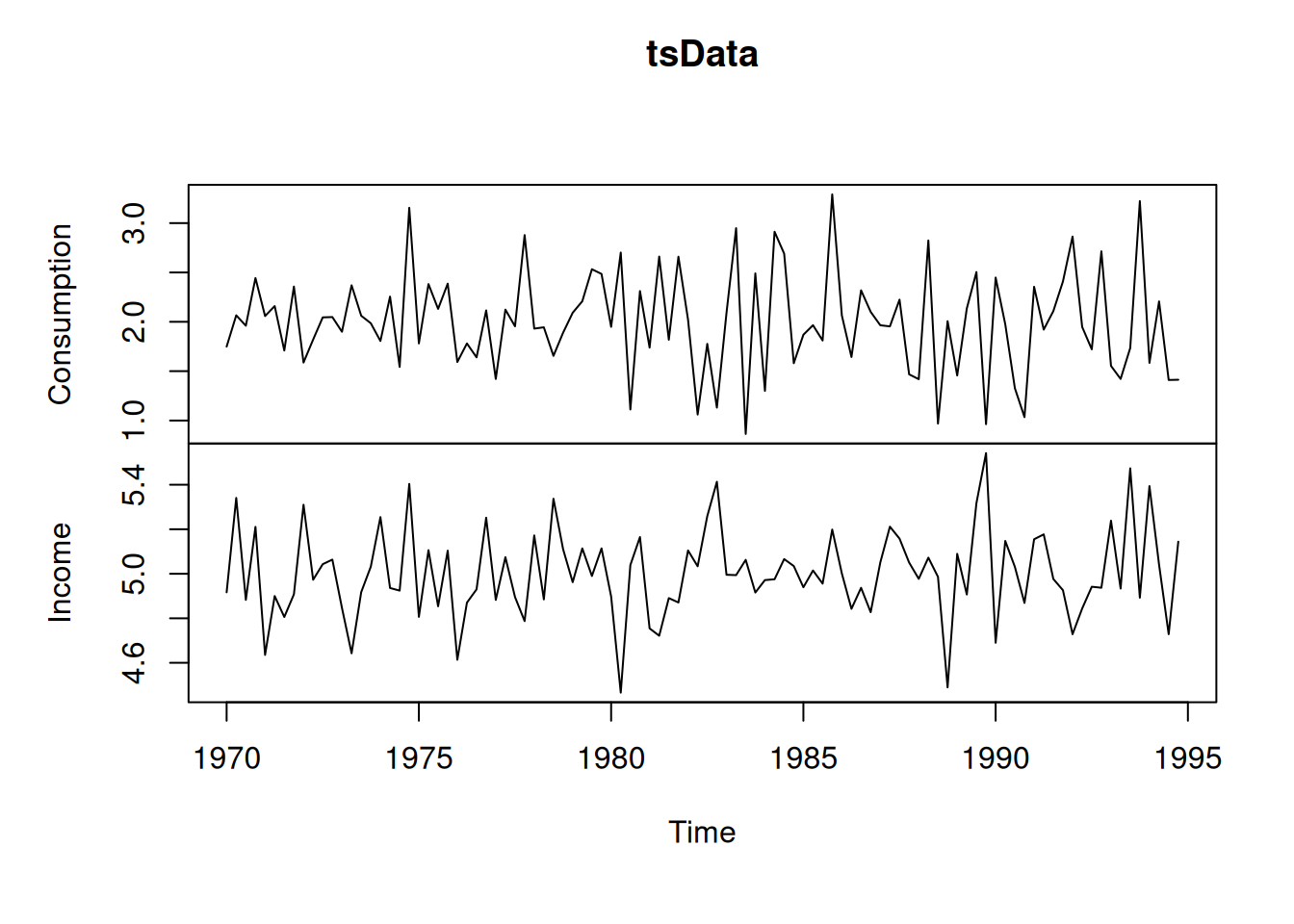
which is different from the case in which the object is a matrix: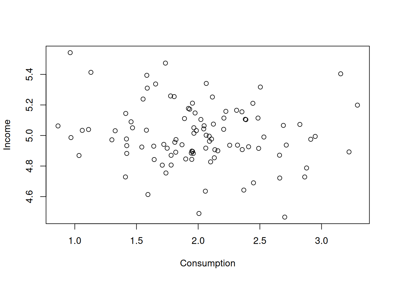
- Higher dimensional arrays: It may sometimes be useful to store information in a matrix with more than 2 dimensions. If we consider the matrix \(B\) above, we could be interested to store the consumption habits of the individuals for two different periods. Suppose \(B\) was the consumption in 1990 and B2, defined bellow is the consumption in 2000. We can define a new matrix containing all the two matrices.
B2 <- matrix(c(250,75,300,250,500,20),2,3)
dimnames(B2) <- dimnames(B2)
allB <- array(0,c(2,3,2))
allB[,,1] <- B
allB[,,2] <- B2
dimnames(allB)[[1]] <- dimnames(B)[[1]]
dimnames(allB)[[2]] <- dimnames(B)[[2]]
dimnames(allB)[[3]]<- c("1990","2000")
allB## , , 1990
##
##      John James Bill
## Book  200   150  100
## Beer  100   150  200
##
## , , 2000
##
## John James Bill
## Book 250 300 500
## Beer 75 250 20