Chapter 3 Linear Equations and Iterative Methods
3.1 Linear algebra
Suppose we want to compute the following problem: \[ Ax=y \] The way we learn how to solve this system in basic textbooks is by inverting \(A\) and multiplying \(y\) by the inverse. In other words, the solution is: \[ x = A^{-1}y \] This solution is right mathematically and has a nice closed-form expression, but is not recommended numerically. Suppose you want to compute the inverse using textbook definition. The number of operations to compute the determinant for an \(n\times n\) matrix is \(O(n!)\). We want to minimize the number of operations and also the number of catastrophic cancellations.
3.1.1 The LU decomposition
The LU decomposition with pivoting is an algorithm developed for that purpose. Pivoting is done to avoid unstable operations and LU decomposition to reduce the number of operations. Consider the following case:
##      [,1] [,2] [,3]
## [1,]    5    8    2
## [2,]    4    6    9
## [3,]    7    3    1
The package “Matrix” includes many algorithms for matrices. Most of the functions produce S4-class objects with information that can only be extracted using the appropriate method. Here is how we obtain L and U (Notice that is is A=PLU, not LU. P is a pivoting matrix):
## 3 x 3 Matrix of class "dtrMatrix"
##          [,1]     [,2]     [,3]
## [1,] 7.000000 3.000000 1.000000
## [2,]        . 5.857143 1.285714
## [3,] . . 7.487805## 3 x 3 sparse Matrix of class "pMatrix"
##
## [1,] . | .
## [2,] . . |
## [3,] | . .## 3 x 3 Matrix of class "dtrMatrix" (unitriangular)
## [,1] [,2] [,3]
## [1,] 1.0000000 . .
## [2,] 0.7142857 1.0000000 .
## [3,] 0.5714286 0.7317073 1.0000000The matrix \(P\) tells us that the the first line of \(A\) is the second line of \(LU\), the second is the third and the third is the first as we can see:
## 3 x 3 Matrix of class "dgeMatrix"
##      [,1] [,2] [,3]
## [1,]    7    3    1
## [2,]    5    8    2
## [3,] 4 6 9## 3 x 3 Matrix of class "dgeMatrix"
## [,1] [,2] [,3]
## [1,] 5 8 2
## [2,] 4 6 9
## [3,] 7 3 1An algorithm to solve the linear model using LU is: (i) first solve Lz=y by recursive substitution, (ii) then solve Ux=z also be recursive substitution. For an \(n\times n\) matrix, the LU decomposition requires \(n^3/3\) floating point operations. The 2 back-substitution algorithms require \(O(n^2)\) operations. For large \(n\), solving a system using LU decomposition is therefore of order \(n^3/3\) (\(n^2\) becomes negligible). We can estimate the order of an algorithm. If we suppose that the time per operation is constant, the estimated time of an algorithm applied to a system of dimension equals to \(n\) can be written as: \[ t_n = Cn^\alpha, \] where \(C\) is a constant (for the LU, \(\alpha=3\)). By applying the algorithm to different \(n\), we can estimate \(\alpha\) using the following regression model: \[ \log{(t_n)} = \alpha_0 + \alpha \log{(n)} +\epsilon_n \] In the following, I estimate the \(\alpha\) for the LU decomposition and Figure 3.1 shows that the relationship is indeed linear.
n <- c(500,1000,1500,2000,2500,3000)
t <- vector()
A <- list()
for (i in 1:length(n))
    A[[i]] <- matrix(rnorm(n[i]^2),n[i],n[i])
for (i in 1:length(n))
    t[i] <- system.time(lu(A[[i]]))[[3]]
ln <- log(n)
lt <- log(t)
print(res<-lm(lt~ln))
##
## Call:
## lm(formula = lt ~ ln)
##
## Coefficients:
## (Intercept) ln
## -2.6635 0.4832plot(lt,ln,type="l",main="Computational time: LU decomposition",
xlab=expression(log(n)),ylab=expression(log(t[n])))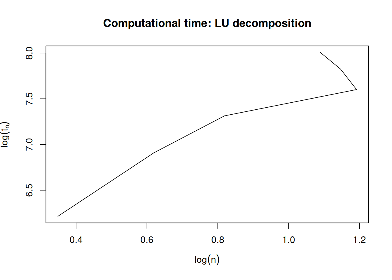
Figure 3.1: Estimated relationship between the dimension of a matrix and its LU decomposition
The estimated coefficient (\(\hat{\alpha}=\) 0.48), is not so far from its true value \(3\). Errors come from the small sample and the fact that time depends not only on operations. Also, computational time may not be constant across operations. But it gives us a good idea. The constant term (\(\hat{\alpha}=\)-2.66) is harder to interpret because it includes the time per operation and the factor of proportionality.
Exercise 3.1 Suppose we want to solve \(Ax=b\) using the following method: (i) invert \(A\) using \(solve(A)\), (ii) obtain the solution using \(x=A^{-1}b\). If we suppose that the number of operation is of order \(O(n^\alpha)\), estimate \(\alpha\).
3.1.2 The Cholesky decomposition
When the matrix \(A\) is symmetric positive definite, there exist a more stable decomposition for which the number of operations is of order \(n^3/6\) (half the number of operations of the LU). It is the Cholesky decomposition. It is a special case of the LU. The decomposition is \(A=LL'\), where \(L\) is a lower triangular matrix. \(L'\) is therefore an upper triangular matrix like \(U\). \(L\) is also called the square root of A. The function chol computes \(L'\):
##      [,1] [,2] [,3]
## [1,]   90   85   53
## [2,]   85  109   73
## [3,] 53 73 86## [,1] [,2] [,3]
## [1,] 9.486833 8.959787 5.586691
## [2,] 0.000000 5.359312 4.281230
## [3,] 0.000000 0.000000 6.038208This decomposition is useful when we work with covariance matrices. If for example the \(n\times 1\) vector \(x\) is \(\sim N(\mu,\Sigma)\), with \(\Sigma=LL'\), x can be written as \(x=\mu+Lz\), where \(z\sim N(0,I)\). The generalized least square method (GLS) is based on the Cholesky decomposition: If \(Var(\epsilon)=\Sigma\) in \(Y=X\beta+\epsilon\), GSL is defined as the OLS applied on the following linear regression model: \[ [L^{-1}Y] = [L^{-1}X]\beta + [L^{-1}\epsilon], \] where again \(\Sigma=LL'\).
3.1.3 The QR decomposition
The last decomposition is called the QR decomposition. It can be applied to any matrix, even if it is not square. Let \(A\) be an \(n\times k\) matrix. The decomposition is \(A=QR\), where \(Q\) is an \(n\times k\) orthogonal matrix (\(Q'Q=I\)) and \(R\) is a \(k\times k\) upper triangular matrix. The rank of \(R\) is equal to the rank of \(A\). If \(A\) is singular, there will be zeros on the diagonal of \(R\). The qr function create an object of class “qr” from which \(Q\) and \(R\) can be extracted using qr.Q and `qr.R respectively. Here is an example:
##            [,1]       [,2]
## [1,] -0.2672612  0.8728716
## [2,] -0.5345225  0.2182179
## [3,] -0.8017837 -0.4364358## [,1] [,2]
## [1,] -3.741657 -8.552360
## [2,] 0.000000 1.963961There is a very useful result when it comes to compute the OLS estimate of \(Y=X\beta+\epsilon\). We can show that all we need is to solve \(Y=X\beta\) using the QR decomposition. The problem to solve is \(Y=QR\beta\), which implies \(Q'Y=R\beta\). Since \(R\) is upper triangular, we can easily solve the problem using back substitutions. The closed-form solution is \(\hat{\beta}=R^{-1}Q'Y\). We can easily show that it is the OLS estimator \((X'X)^{-1}X'Y\), that the projection matrix is \(P_x=QQ'\) and the residuals \((I-QQ')y\).
Exercise 3.2 Write a function that computes the solution to \(Ux=b\) where \(U\) is upper triangular. The function will be backSub(U,b). Make sure the function checks whether \(U\) is triangular of not. The solution must be done using the back substitutions. Loops may therefore be required in that case.
Exercise 3.3 Write the function myQrlm(Y,X), that returns the OLS estimators, the standard errors, the t-test and the p-values all in the same matrix with the appropriate names for the columns and the rows. You have to use the QR decomposition and the function you wrote in the previous exercise. You are not allowed to compute X’X, X’Y and to use the solve function to compute inverses.
In a problem in which we need to solve \(f(x)=0\), we want to measure the stability of the solution when the system is perturbed. In the linear system \(Ax=b\), \(f(x) = Ax-b\) and the solution is \(x=A^{-1}b\). If \(b\) is subject to the rounding errors \(r\), the solution to the perturbed system is \(\tilde{x}=A^{-1}b+A^{-1}r\). The condition number is defined as: \[ Cond = \frac{\frac{\|x-\tilde{x}\|}{\|x\|}}{\frac{\|r\|}{\|b\|}}= \frac{\|A^{-1}r\|}{\|x\|}\frac{\|b\|}{\|r\|} \] If we define the condition number of A as \(Cond(A)=\|A\|\|A^{-1}\|\), the above condition number is bound above by \(Cond(A)\) and bellow by \(1/Cond(A)\). A condition number of C implies that the solution is subject to an error of approximately C times larger than the rounding error (in percentage). The condition number of a matrix can be approximated by the ratio of its largest eigenvalue (\(\lambda_{max}\)) to its smallest one (\(\lambda_{min}\)). In fact \(\lambda_{max}\) is an upper bound for \(\|A\|\) and \(1/\lambda_{min}\) an upper bound for \(\|A^{-1}\|\) Consider the following OLS problem (here I use \((X'X)^{-1}X'Y\) to illustrate multicolinearity):
set.seed(123)
x <- cbind(1,2,rnorm(40))
x[20,2] <- 2.0001
XX <- t(x)%*%x
XY <- c(1,2,3)
ev <- eigen(XX)$value
condNum <- max(ev)/min(ev)
condNum
## [1] 103520161296The condition number of \(X'X\) is huge. We can see that the impact of a small variation of \(X'Y\) can have a large effect on \(\hat{\beta}\):
## [1] -490.19805943 245.10909062 0.09440253## [1] -2.559599e+03 1.279808e+03 9.610748e-02The problem of multicolinearity is a problem with the stability of the linear system \((X'X)\beta = (X'Y)\) caused by the near singularity of \(X'X\). There is a way of stabilizing the solution. We can regularize the solution by adding a small positive number to the diagonal of \(X'X\). In the OLS case, it is called “Ridge Regression”. In a general problem \(Ax=b\), it is called a regularized technique. We can see the impact of adding .01 to the diagonal of \(X'X\) in our problem:
## [1] 20010.72## [1] 0.004055934 0.008348604 0.093968818## [1] 0.003655954 0.008548644 0.093968813The problem is of course to find the appropriate regularization parameter.
3.2 Iterative method
In this section, we give an introduction to iterative methods. In this section, it is only applied to the case of linear problems such as \(Ax=b\). However, we will use similar methods in next chapters for solving nonlinear system of equations and to do numerical optimization. I only present here examples:
3.2.1 Stopping rules
Lets consider the computation of \(e^x=\sum_{n=0}^\infty x^n/n!\). Obviously, we can not compute the exact value. We need to stop somewhere. What criterion should we use to consider our answer to be reasonably good? Table 3.1 gives us a measure of the error as a function of \(n\):
x <- 1
n <- c(0:8)
myExp <- cumsum((x^n)/factorial(n))
Exp <- exp(x)
er <- abs(myExp-Exp)
err <- er/Exp
ans <- cbind(n,myExp,Exp,er,err)
colnames(ans) <- c("n","My Exp", "True Exp","Abs Error","Rel Error")| n | My Exp | True Exp | Abs Error | Rel Error |
|---|---|---|---|---|
| 0 | 1.00000 | 2.71828 | 1.71828 | 0.63212 |
| 1 | 2.00000 | 2.71828 | 0.71828 | 0.26424 |
| 2 | 2.50000 | 2.71828 | 0.21828 | 0.08030 |
| 3 | 2.66667 | 2.71828 | 0.05162 | 0.01899 |
| 4 | 2.70833 | 2.71828 | 0.00995 | 0.00366 |
| 5 | 2.71667 | 2.71828 | 0.00162 | 0.00059 |
| 6 | 2.71806 | 2.71828 | 0.00023 | 0.00008 |
| 7 | 2.71825 | 2.71828 | 0.00003 | 0.00001 |
| 8 | 2.71828 | 2.71828 | 0.00000 | 0.00000 |
We can obtain the convergence rate by looking at the behaviour of \(\|x_{n+1}-x\|/\|x_n-x\|\) (see Figure 3.2):
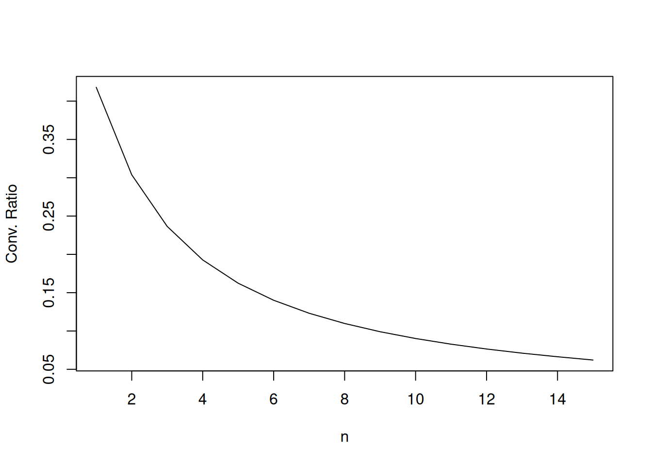
Figure 3.2: The convergence ratio \(\|x_{n+1}-x\|/\|x_n-x\|\) as a function of \(n\)
A sequence converge linearly if: \[ \lim_{n\rightarrow \infty} \frac{\|x_{n+1}-x\|}{\|x_n-x\|} \leq \beta < 1 \] and super-linearly (or at a rate \(q>1\)) if \(\beta=0\). A general rule can be obtained by assuming that the above inequality is true which implies that: \[ \|x_{n+1}-x_n\| \geq \|x_n-x\|(1-\beta) \] Therefore, a rule that says: stops at \(x_{n+1}\) if \(\|x_{n+1}-x_n\|<\epsilon (1-\beta)\) implies an error bounded by \(\|x_n-x\|<\epsilon\). For our case, it seems that the sequence to compute the exponential is superlinear (the ratio converges to zero) which implies that we can use the following function, which include the stopping rule. We can see that \(\epsilon\) is just an upper bound for the error:
myExp <- function(x,eps)
    {
    y0 <- 1
    n <- 1
    crit <- 1000
    while(crit>eps)
        {
        y <- y0+(x^n)/factorial(n)
        crit <- abs(y-y0)
        n <- n+1
        y0 <- y
        }
    return(y)
}## [1] 6.138994e-05## [1] 4.142358e-10## [1] 4.618528e-14Sometimes we also see rules based on the relative variation of the \(x_n\). This rule is: stop at \(x_{n+1}\) if \(\|x_{n+1}-x_n\|/(1+\|x_n\|)\leq \epsilon\). The value in the denominator is to allow convergence to zero. This rule however does not work well with sequences that converge linearly. We can see that using the sequence \(x_n = \sum_{i=1}^n (1/i)\):
N <- 100
n <- 1:N
x <- sum(1/n)
xn <- cumsum(1/n[-N])
y <- abs(xn[-1]-x)/abs(xn[-length(xn)]-x)
beta <- max(y)
beta
## [1] 0.973315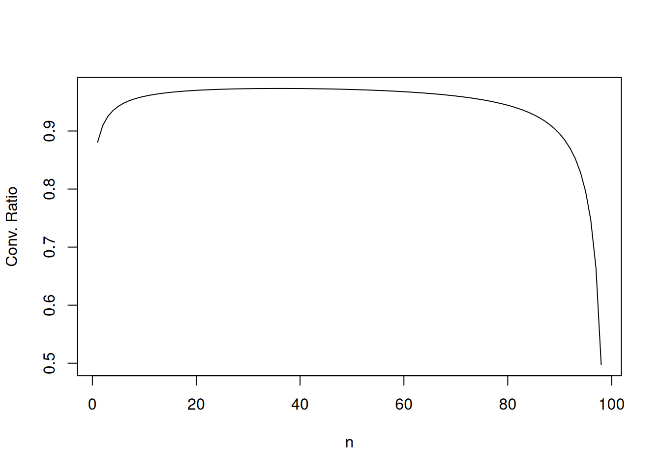
Figure 3.3: The convergence ratio \(\|x_{n+1}-\hat{x}\|/\|x_n-\hat{x}\|\) as a function of \(n\) for \(x_n=\sum_i (1/i)\)
In Figure 3.3 we can see that \(\beta\) as an upper bound around 1, which shows that there is no convergence. Using the first rule we would never conclude that the sequence converges.
3.2.2 Fixed-Point Iteration
If we define \(G(x)=Ax-b+x\), the solution to \(Ax=b\) is the fixed-point \(G(x)=x\). The following iteration, if it converges, will reach the solution: \[ x_{k+1} = G(x_k) = (A+I)x_k-b \] Lets try it:
FP <- function(A,b,x0,eps,maxit=1000,beta=0)
    {
    crit <- 1000
    n <- 1
    while(crit>eps*(1-beta))
        {
        x <- (A+diag(ncol(A)))%*%x0-b
        crit <- sqrt(crossprod(x-x0))
        x0 <- c(x)
        n <- n+1
        if (n>=maxit | any(abs(x)==Inf))
            {
            warning("No convergence")
            break
            }
        }
    return(x)
    }
A <- matrix(c(12,3,2,5,13,7,4,9,10),3,3)
b <- c(4,5,6)
trueX <- solve(A,b)
FP(A,b,c(0,0,0),1e-6)
## Warning in FP(A, b, c(0, 0, 0), 1e-06): No convergence## [,1]
## [1,] -Inf
## [2,] -Inf
## [3,] -InfNo luck! It does not converge. This method is quite bad because we have convergence only if the modulus of the eigenvalues of \((A+I)\) are less than 1. The following example works.
A <- matrix(c(-.2,.1,.1,.3,-.3,.3,.4,-.1,-.6),3,3)
Tx <- solve(A,b)
x <- FP(A,b,c(10,10,10),1e-5,maxit=5000)
crossprod((Tx-x))^.5
## [,1]
## [1,] 0.00101769## [,1]
## [1,] 1.017961e-06The error is however higher than \(\epsilon\) when \(\beta=0\). The convergence is therefore linear. We need a \(\beta\) close to 1 for the error to be bounded by \(\epsilon\):
##              [,1]
## [1,] 5.080091e-06## [,1]
## [1,] 5.07855e-093.2.3 Gauss-Jacobi and Gauss-Seidel
Here I reproduce Figure 3.2 of Judd (1998). First I need to build few functions.
# Did I tell you I like small functions?
getXiGJ <- function(A,b,x)
        {
        a <- diag(A)
        diag(A) <- 0
        x <- (b-A%*%x)/a
        attr(x,"name") <- "Gauss-Jacobi"
        return(x)
        }
getXiGS <- function(A,b,x)
        {
        xf <- rep(0,length(x))
        a <- diag(A)
        diag(A) <- 0
        for (i in 1:length(x))
            x[i] <- (b[i]-crossprod(A[i,],x))/a[i]
        attr(x,"name") <- "Gauss-Seidel"
        return(x)
    }
# The function prepares A so that the diagonals are not zero
PrepA <- function(A,b)
    {
    bad <- which(abs(diag(A))<=1e-7)
    for (i in bad)
        {
        l <- which(abs(A[,i])>1e-7)
        if (length(l)==0)
            return(list(A=NULL,b=NULL,fail=TRUE))
        A[i,] <- A[i,]+A[l[1],]
        b[i] <- b[i]+b[l[1]]
        }
    return(list(A=A,b=b,fail=FALSE))
  }
# This function works for both algorithm
IterSolve <- function(A,b,x0,algo,eps=1e-8,maxit=1000,...)
  {
  res <- PrepA(A,b)
  if(res$fail)
    stop("The algorithm failed")
  else
    {
    A <- res$A
    b <- res$b
    }
  crit <- 1000
  AllX <- x0
  n <- 1
  while(crit>eps)
    {
    x <- c(algo(A,b,x0,...))
    AllX <- rbind(AllX,x)
    if (any(abs(x)==Inf))
          stop("The algorithm diverges")
      crit <- crossprod(x-x0)^.5
      if (n == maxit)
        {
        warning("Maxit reached")
          break
        }
    n <- n+1
      x0 <- x
      }
  if (n<maxit)
    cat("\n",attr(x,"name"),"\nConverged after ", (n-1), "iterations\n")
  return(list(x=x,AllX=AllX))
  }
We can try it with the previous matrix
##
##
## Converged after  399 iterations
## [1] -959.9998 -239.9999 -289.9999##
##
## Converged after 169 iterations## [1] -959.9999 -240.0000 -290.0000The second method is clearly faster than the first method, which is explained by the fact that it uses the new information as soon as it is available. The two methods are also much faster than the Fixed-point method. They also seem to converge better since they both can solve the first problem we tried above with the Fixed-Point algorithm. To see it, we even try very bad starting values:
A <- matrix(c(12,3,2,5,13,7,4,9,10),3,3)
b <- c(4,5,6)
IterSolve(A,b,c(100,-100,50),eps=1e-5,algo=getXiGJ)$x
##
##
## Converged after 104 iterations## [1] 0.16021871 -0.08840049 0.62983159##
##
## Converged after 22 iterations## [1] 0.16022332 -0.08840292 0.62983738But there are examples in which the algorithms do not converge:
set.seed(111)
A <- matrix(rnorm(9),3,3)
x1 <- try(IterSolve(A,b,c(100,-100,50),eps=1e-5,algo=getXiGS))
## Error in IterSolve(A, b, c(100, -100, 50), eps = 1e-05, algo = getXiGS) :
## The algorithm diverges## Error in IterSolve(A, b, c(100, -100, 50), eps = 1e-05, algo = getXiGS) :
## The algorithm divergesWe’ll comeback to this convergence problem latter. We first want to see how we can use the algorithm to analyze the dynamics of market going from any point to the equilibrium. The model is: \[ p+q=10~~~\mbox{(demand)} \] \[ p-2q=-2~~~\mbox{(supply)} \] or \[ \begin{pmatrix} 1&1\\1&-2 \end{pmatrix} \begin{pmatrix} p\\q \end{pmatrix}= \begin{pmatrix} 10\\-2 \end{pmatrix} \] First lets compare the two methods:
##
##
## Converged after 21 iterations##
##
## Converged after 40 iterationsans <- cbind(1:20,res1$AllX[1:20,],res2$AllX[1:20,])
colnames(ans) <- c("n","p-(GS)","q-(GS)","p-(GJ)","q-(GJ)")Table 3.2 shows some iteration results. We can see that the Gauss-Seidel method is faster. The function plotEqui() creates something similar to Figure 3.2 of Judd. The result is shown in Figure 3.4. The Gauss-Seidel method is slightly different because we solve for the price first while Judd does the opposite. Also, the path in the book shows movements between iteration while here we only show the final points.
| n | p-(GS) | q-(GS) | p-(GJ) | q-(GJ) |
|---|---|---|---|---|
| 1 | 4.0000 | 1.0000 | 4.0000 | 1.0000 |
| 2 | 9.0000 | 5.5000 | 9.0000 | 3.0000 |
| 3 | 4.5000 | 3.2500 | 7.0000 | 5.5000 |
| 4 | 6.7500 | 4.3750 | 4.5000 | 4.5000 |
| 5 | 5.6250 | 3.8125 | 5.5000 | 3.2500 |
| 6 | 6.1875 | 4.0938 | 6.7500 | 3.7500 |
| 7 | 5.9062 | 3.9531 | 6.2500 | 4.3750 |
| 8 | 6.0469 | 4.0234 | 5.6250 | 4.1250 |
| 10 | 6.0117 | 4.0059 | 6.1875 | 3.9375 |
| 15 | 5.9996 | 3.9998 | 6.0156 | 4.0234 |
| 20 | 6.0000 | 4.0000 | 5.9941 | 4.0020 |
plotEqui <- function(resGS,resGJ,A,b,n, Title=NULL,xlab=NULL,ylab=NULL)
    {
    x <- resGS$AllX[1:n,]
    x2 <- resGJ$AllX[1:n,]
    xsol <- solve(A,b)
    xlim <- c(0,2*xsol[2])
    ylim <- c(0,2*xsol[1])
    if (is.null(xlab))
            xlab <- "Q"
    if (is.null(ylab))
            ylab <- "P"

    curve((b[1]-A[1,2]*x)/A[1,1],0,xlim[2],xlim=xlim,
                ylim=ylim,xlab=xlab,ylab=ylab,bty="n")
    abline(b[2]/A[2,1],-A[2,2]/A[2,1])
    if (is.null(Title))
        title("Dynamics of Demand and Supply Equilibrium")
    else
        title(Title)
    for (i in 1:(n-1))
            {
            text(x[i,2],x[i,1],i,col=2,lwd=4)
            arrows(x[i,2],x[i,1],x[(i+1),2],x[(i+1),1],col=2)
            }
    text(x[n,2],x[n,1],n,col=2,lwd=4)
    for (i in 1:(n-1))
            {
            text(x2[i,2],x2[i,1],i,col=4,lwd=4)
            arrows(x2[i,2],x2[i,1],x2[(i+1),2],x2[(i+1),1],lty=2,col=4)
            }
    text(x2[n,2],x2[n,1],n,col=4,lwd=4)
    legend("top",c("Gauss-Seidel","Gauss-Jacobi"),lty=c(1,1),col=c(2,4))
    }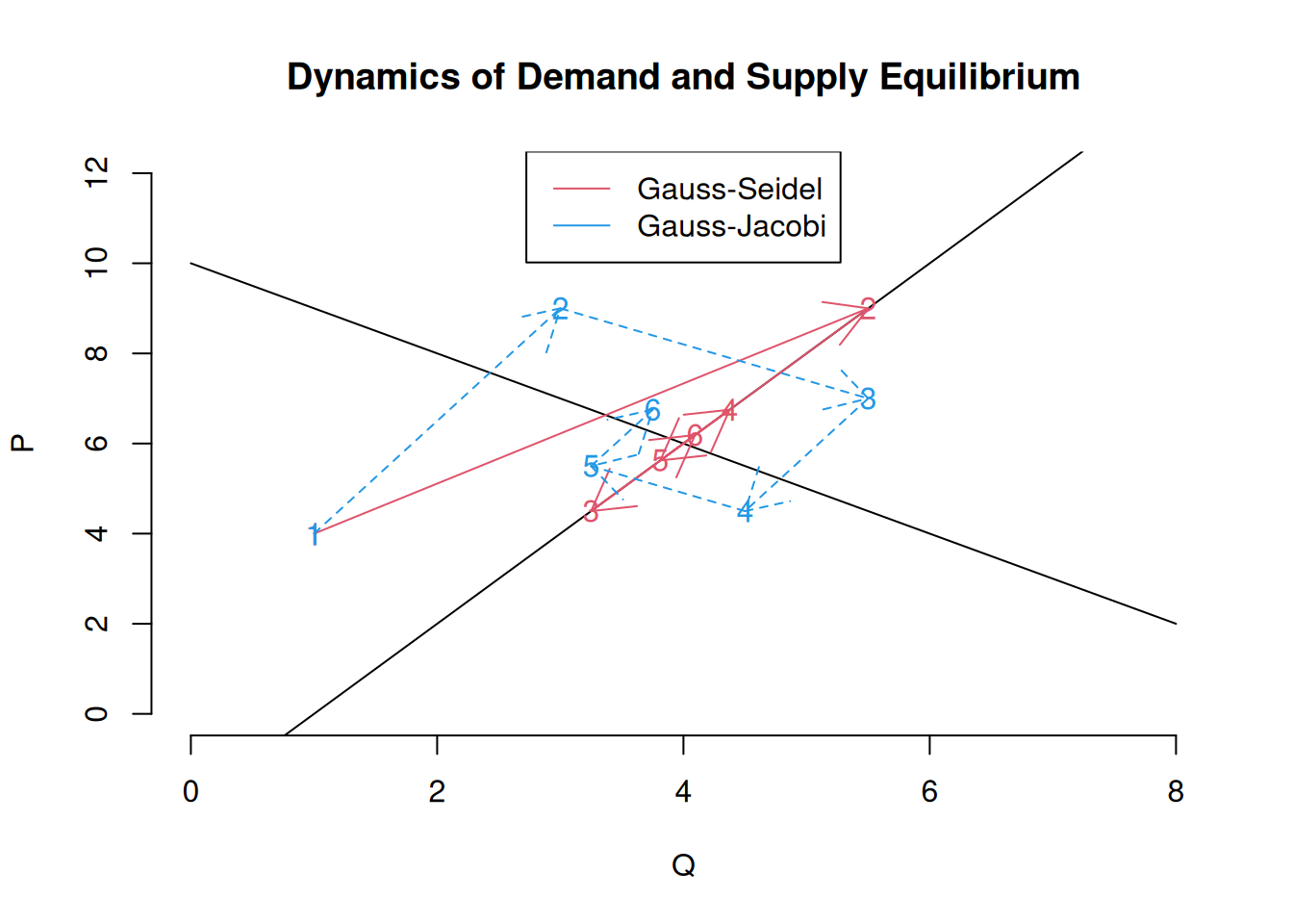
Figure 3.4: Dynamics of the market using two types of iterative methods
Using the dynamics of the model, we can see why in some cases, the iterative procedure does not converge. It is a nice example that uses the same argument as when we analyze movements in differential equation models graphically. The method converges because of the angle between the demand and the supply around the equilibrium. Figure 3.5 shows what happens if the slope of the demand becomes -2.1:
A <- matrix(c(1,1,2.1,-2),2,2)
b <- c(10,-2)
res1 <- IterSolve(A,b,c(2.2,3.8),eps=1e-5,algo=getXiGS)
## Warning in IterSolve(A, b, c(2.2, 3.8), eps = 1e-05, algo = getXiGS): Maxit
## reached## Warning in IterSolve(A, b, c(2.2, 3.8), eps = 1e-05, algo = getXiGJ): Maxit
## reached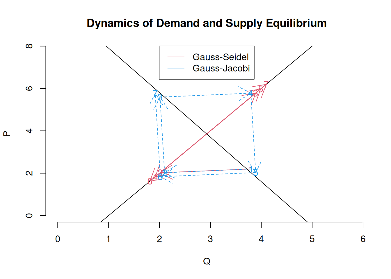
Figure 3.5: Dynamics of the market using two types of iterative methods
We would get a perpetual cycle if the ratio was 1 in absolute value (try it). Here we are just solving a linear system. The non-convergence of the iterative methods does not imply that we do not have a solution:
## [1] 3.853659 2.926829The problem comes from the algorithm not the system itself. However, if we had a dynamic system, the system would be considered unstable. We’ll cover that later.
There is a general rule for the convergence of both algorithms. If A is diagonally dominant \((|a_{ii}|>\sum_{j \neq i} |a_{ij}|)\) , the method works. We can construct diagonally dominant matrices from one that is not diagonally dominant. For example, if the first row of A is replaced by the sum of the first and the second we get (we have to do the same transformation to b):
##      [,1] [,2]
## [1,]    2  0.1
## [2,]    1 -2.0
The matrix becomes diagonally dominant. The system can therefore be solved:
##
##
## Converged after  5 iterations
## [1] 3.853659 2.926829##
##
## Converged after 9 iterations## [1] 3.853659 2.926829Of course it make no sense economically to replace the demand by the sum of the demand and the supply. It is just a numerical trick to make the algorithm works.
Exercise 3.4 Rewrite the function PrepA so that (if possible) all rows of A becomes diagonally dominant.
3.2.4 Acceleration and Stabilization Methods
We first rewrite the function getXiGJ and getXiGS to include the parameter \(\omega\) of the altered iterative scheme, with default value of 1.
getXiGJ <- function(A,b,x,omega=1)
        {
        a <- diag(A)
        diag(A) <- 0
        x <- omega*(b-A%*%x)/a + (1-omega)*x
        attr(x,"name") <- "Gauss-Jacobi"
        return(x)
        }

getXiGS <- function(A,b,x,omega=1)
        {
        xf <- rep(0,length(x))
        a <- diag(A)
        diag(A) <- 0
        for (i in 1:length(x))
            x[i] <- omega*(b[i]-crossprod(A[i,],x))/a[i]+(1-omega)*x[i]
        attr(x,"name") <- "Gauss-Seidel"
        return(x)
        }
Lets try to solve our previous unstable system using this modified iterative scheme:
A <- matrix(c(1,1,2.1,-2),2,2)
b <- c(10,-2)
resGS <- IterSolve(A,b,c(2.2,3.8),eps=1e-5,algo=getXiGS,omega=.7)
##
##
## Converged after 12 iterations##
##
## Converged after 49 iterationsFigure 3.6 shows what happens. The problem was that the steps were to large. By reducing them, we obtain convergence. In the case of a slow convergence, we can also use \(\omega\) to accelerate convergence. The following system is an example in which convergence is very slow: \[ p =-1.95q+10 \] \[ q=2q-2 \] Figure 3.7 shows the convergence when \(\omega=1\) and Figure 3.8 shows what happens if we set \(\omega\) to 0.6.
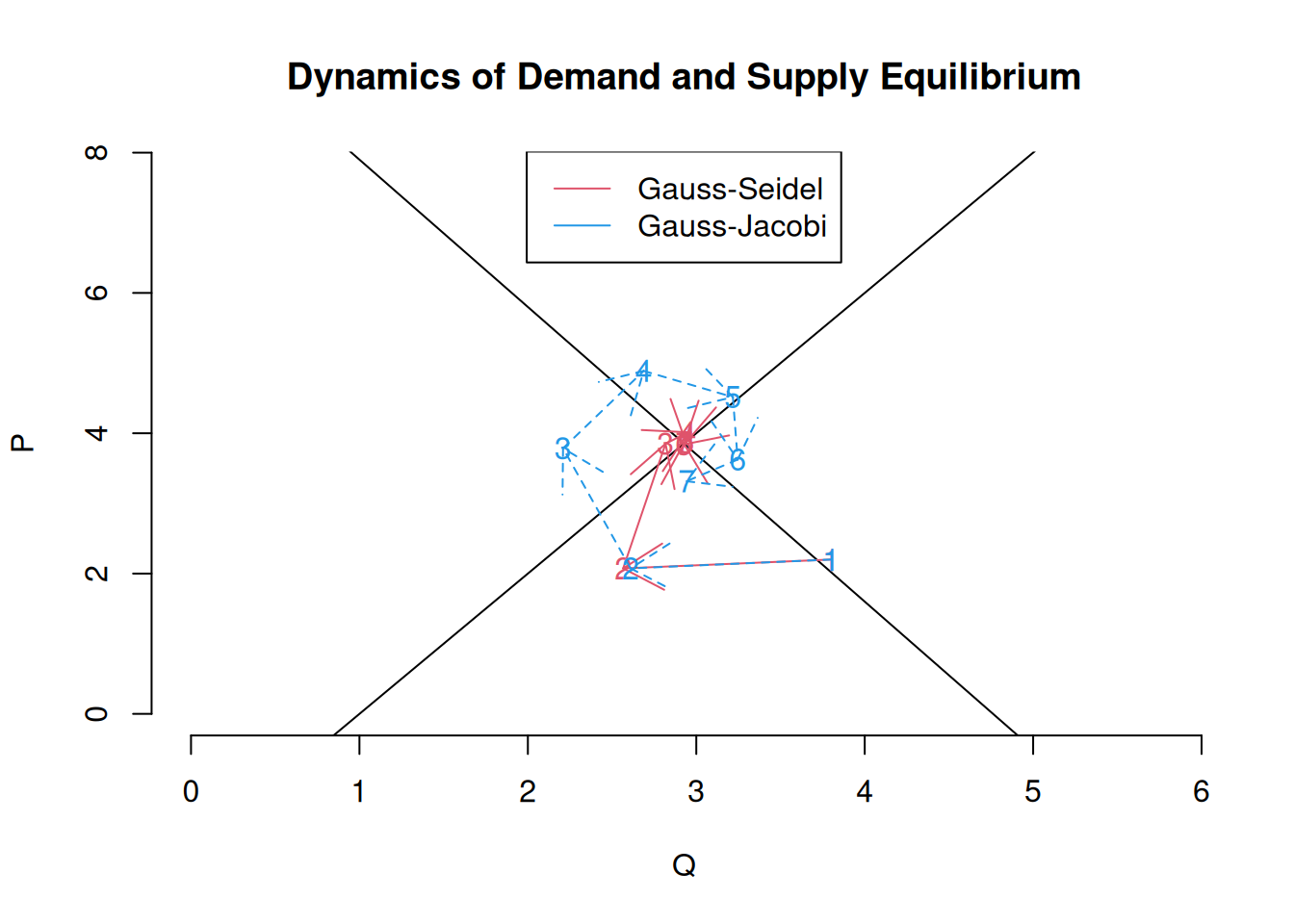
Figure 3.6: Gauss-Seidel and Gauss-Jacobi using an altered scheme
##
##
## Converged after 504 iterations##
##
## Converged after 955 iterations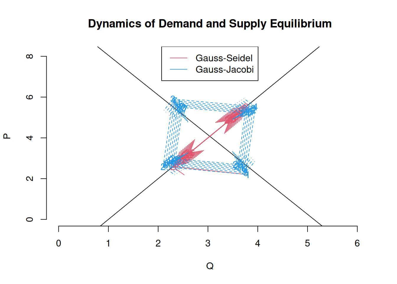
Figure 3.7: Gauss-Seidel and Gauss-Jacobi using an altered scheme (Slow convergence with \(\omega=1\)
##
##
## Converged after 14 iterations##
##
## Converged after 36 iterations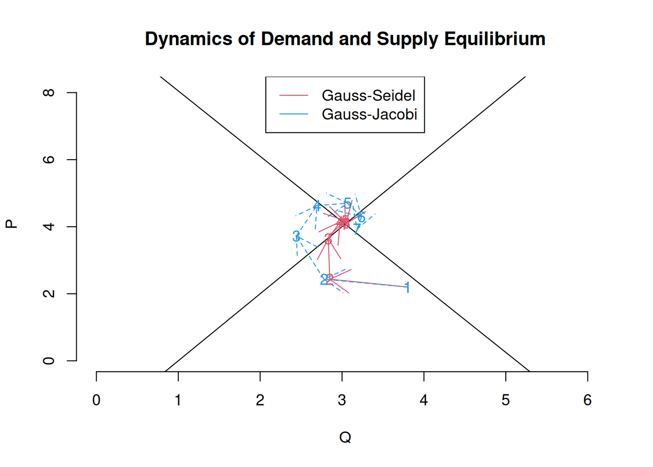
Figure 3.8: Gauss-Seidel and Gauss-Jacobi using an altered scheme (Slow convergence with \(\omega=0.6\)
For Gauss-Seidel, we can obtain an optimal \(\omega\). If we write the iteration in matrix form, we have: \[ x_{k+1} = M_\omega^{-1}N_\omega x_k+\omega M_\omega^{-1} b \] where \(M_\omega=(D+\omega L)\), \(M_\omega=(1-\omega)D-\omega U\), and \(U\), \(L\), and \(D\) are respectively the element above the diagonal, the element below the diagonal and the diagonal of \(A\). In fact, we have \(A=U+L+D\). The iterative scheme converges quickly if the largest eigenvalues of \(( M_\omega^{-1}N_\omega)\) in absolute value is small and less than 1. We therefore what the value of \(\omega\) that minimizes the largest eigenvalues. The following function selects the optimal \(\omega\) using a grid search. It is not efficient but it works:
getOmega <- function(A,from=.1,to=1)
    {
    w <- seq(to,from,len=100)
    ev <- vector()
    D <- diag(diag(A))
    U <- A*upper.tri(A)
    L <- A*lower.tri(A)
    for (i in 1:length(w))
        {
        M <- D+w[i]*L
        N <- (1-w[i])*D-w[i]*U
        ev[i] <- max(abs(eigen(solve(M,N))$val))
        }
    w[which.min(ev)]
    }
We can verify with the last two systems:
A <- matrix(c(1,1,2.1,-2),2,2)
b <- c(10,-2)
w <- getOmega(A,0,3)
res1 <- IterSolve(A,b,c(2.2,3.8),eps=1e-5,algo=getXiGS,omega=w)
##
##
## Converged after 9 iterationsA <- matrix(c(1,1,1.95,-2),2,2)
w <- getOmega(A,0,3)
resGS <- IterSolve(A,b,c(2.2,3.8),eps=1e-5,algo=getXiGS,omega=w)##
##
## Converged after 10 iterationsIt is in fact very fast with the optimal \(\omega\).
Exercise 3.5 Try to find the optimal \(\omega\) for the Gauss-Jacobi method and write a function like the one above to compute it. Compare the convergence of Gauss-Seidel and Gauss-Jacobi using their optimal \(\omega\).
Exercise 3.6 Do the same for the fixed point algorithm.
We conclude this chapter with an example of Nash equilibrium computation. The two reaction functions are: \[ p_1=1+0.75 p_2 \] \[ p_2 =2+0.8p_1 \] In the following, we compare the convergence with different \(\omega\) (find the optimal one), and Figure 3.9 shows the case \(\omega=1\).
##
##
## Converged after 27 iterations##
##
## Converged after 50 iterations##
##
## Converged after 78 iterations##
##
## Converged after 96 iterationsIn this example, reducing the value of \(\omega\) does not help. Figure 3.10 shows us why. In fact, we can accelerate the convergence by choosing a value greater than 1.
##
##
## Converged after 13 iterations## Warning in IterSolve(A, b, c(2, 1), eps = 1e-05, algo = getXiGJ, omega = 1.3):
## Maxit reachedIt works for the Gauss-Seidel but not for the Gauss-Jacobi, which shows that the optimal \(\omega\) is not the same for the two algorithms. You can use the answer of Exercise 3.5 to show it.
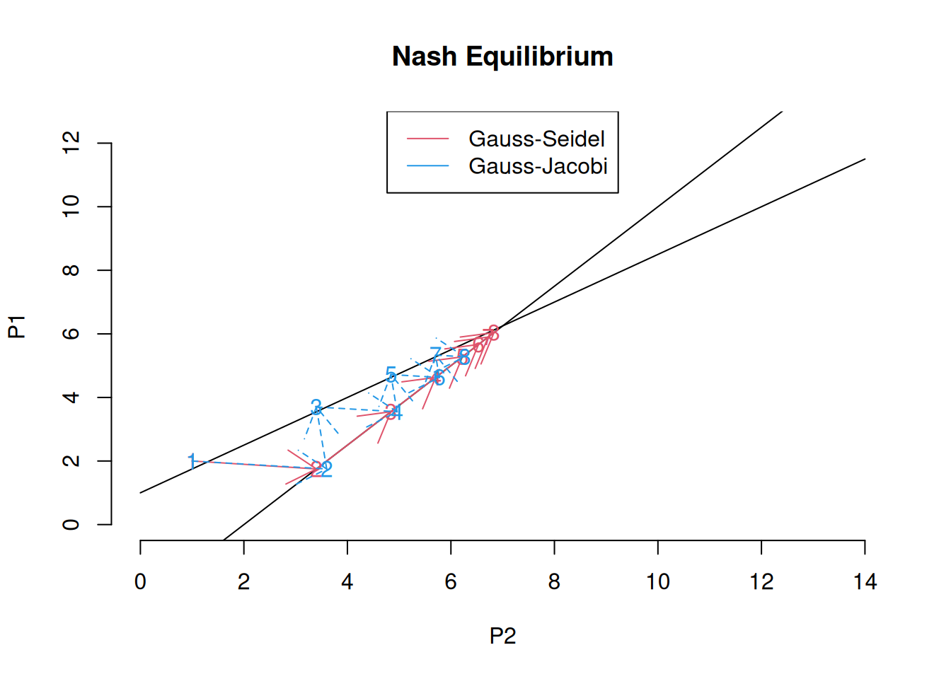
Figure 3.9: Gauss-Seidel and Gauss-Jacobi for the computation of a Nash equilibrium (\(\omega=1\))
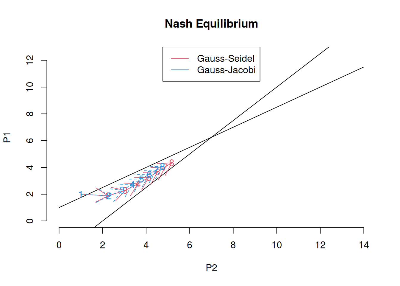
Figure 3.10: Gauss-Seidel and Gauss-Jacobi for the computation of a Nash equilibrium (\(\omega=0.5\))
Exercise 3.7 Answer questions 3, 6, 7 and 8 in Judd