Chapter 8 Differential Equations
8.1 Introduction
In this chapter, we are interested in problems that can be written as: \[\begin{equation} \frac{dy}{dx} = f(x,y)\,, \tag{8.1} \end{equation}\] where \(x\in [a,b]\), \(y\in \mathbb{R} ^n\), and \(f: \mathbb{R} ^{n+1}\rightarrow \mathbb{R} ^n\). This is called a system of first order “Ordinary Differential Equation” (ODE). This is a very general representation of differential equations because higher order equations can always be redefined as a first order equation be an appropriate change of variable. For example, the second order differential equation \(y''(x) = f(y'(x),y,x)\) can be written as a system of two first order differential equations: \(z'(x) = f(z,y,x)\), and \(y'(x)=z\). The goal is to obtain the solution \(y(x)\) that satisfies equation (8.1).
For example, consider the following simple Solow Growth model: \[\begin{equation}\begin{split} \dot{k} \equiv \frac{dk}{dt} = & sf(k)-\delta k\\ f(k) = &k^\alpha \end{split} \tag{8.2} \end{equation}\] This is a special case of equation (8.1) with \(x=t\in[0,\infty]\), \(y=k\), and \(f(t,k)=sk(t)^\alpha-\delta k(t)\). Before going through numerical methods to solve ODE’s, lets see how we can solve it analytically. I am not going into all possible cases. I just want to give you some notions. First, there is no analytical solution to the problem (8.2). We can write: \[ k(t) = k(0) + \int_0^t[sk(t)^\alpha-\delta k(t)] dt, \] but we cannot solve it because we don’t know the function \(k(t)\). Second, we need more information in order to find \(k(t)\). The ODE only informs us about the behavior of the derivative \(\dot{k}\). Finding \(k(t)\) only based on the problem (8.2) is like finding \(x_t=f(t)\) based only on \((x_{t+1}-x_t)=a\). However, if we know that \(x_0=c\), we can obtain \(x_t=x_0+at\). Solutions to nonlinear differential equations only exist in closed form for a few cases.
Lets consider a simpler case: \[ y'(x) = ay(x) + b, \] where \(a<0\). The solution of differential equation, as it is also the case for difference equations, has two parts: a complementary solution \(S_c\) and a particular solution \(S_p\). To first is obtained by solving the homogeneous version of the ODE, \(y'(x)=ay(x)\), and the second is the solution for a particular value of \(x\), which is often the steady state value, \(-b/a\). We can write the homogeneous part of the ODE as: \[ \frac{dy}{y} = adx \] If we integrate both side, we obtain: \[ \begin{split} \int \frac{dy}{y} = & \int adx\\ \log(y) =& ax + C\\ S_c = Ce^{ax} \end{split} \] It implies that the general solution is \(y(t) = Ce^{at}-b/a\). The final solution is obtained by setting \(y(x)\), for \(x\in[a,b]\), to some value \(y_0\), which gives the value of the integrating constant \(C=y_0+b/a\). The solution is therefore: \[ y(t) = \left(y_0+\frac{b}{a}\right)e^{at} - \frac{b}{a} \] For nonlinear equations, there are special cases for which solutions can be found. For example, if the ODE can be written as \(f(y)dy=g(x)dx\), in which case we say that the variables are separable, we can solve it by integrating both sides. However, separable variables is not a sufficient condition for the closed form solution to exist. For example, the Solow model can be written as: \[ \int \frac{1}{sk^\alpha-\delta k} dk = t + C, \] but even if the integral exists, we cannot isolate \(k(t)\). The problem with solving differential equations is like the problem of integrating. The best method is determined on a case by case basis. Fortunately, we have easier numerical methods to solve any ODE.
8.2 Finite Difference Methods for initial value problems
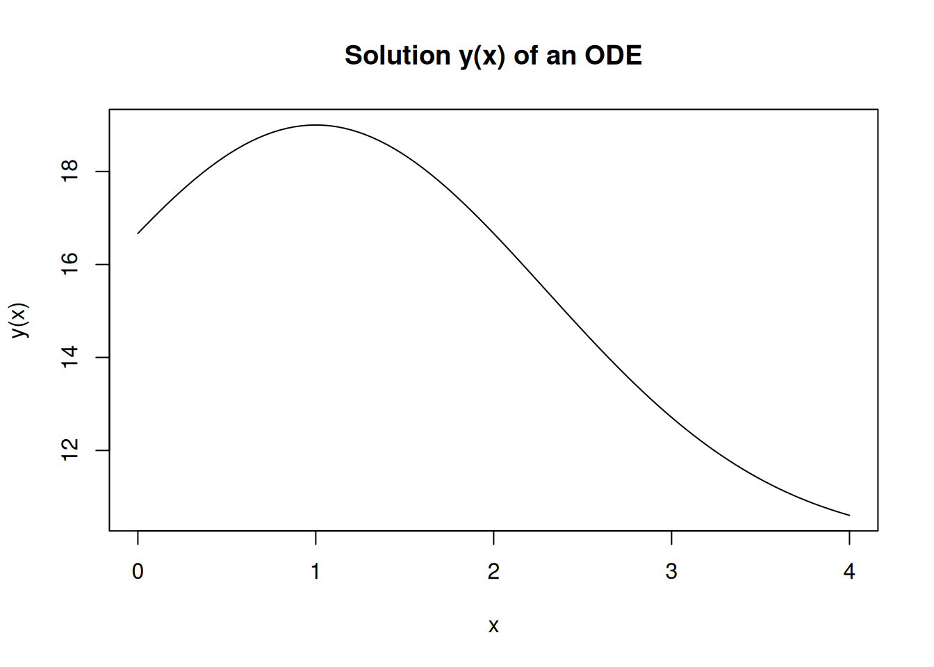
Lets consider the following ODE: \[\begin{equation} \frac{dy}{dx} = -0.6 (y-10)(x-1) \tag{8.3} \end{equation}\] with \(y(0)=9e^{-0.3}+10\). It is a weird starting value that produce a nice solution: \[ y(x) = 9e^{-0.3(x-1)^2} + 10 \] The following graph shows the solution of the ODE:
8.2.1 Euler’s Method
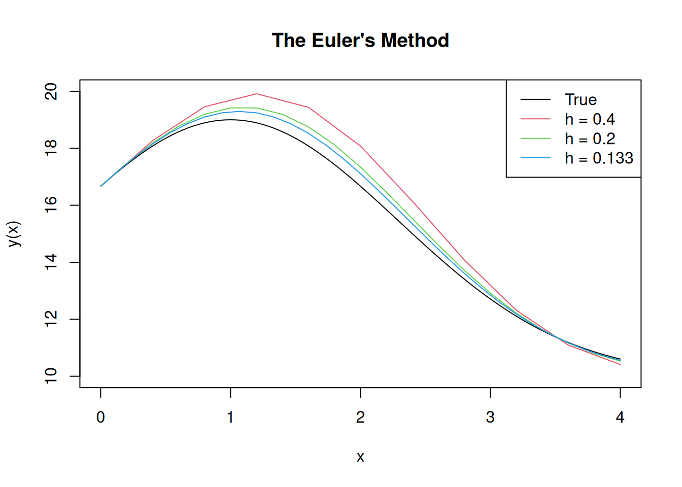
Lets consider the general case: \[ y'(x) = f(x,y), \] for \(x\in[a,b]\), and \(y(a)=y_0\). Lets consider \(n+1\) points \(x_i\), \(i=0,...,n\), such that \(x_i = a+ih\), where \(h\) is the step size. The Euler’s method is based in the result: \[ y(x_{k+1})-y(x_k) = \int_{x_k}^{x_{k+1}} f(x,y(x)) dx \] By the rectangle rule, the right hand side can be approximated by \(hf(x_k,y(x_k))\), which gives us the Euler’s algorithm: \[ y_{k+1} = y_{k} + hf(x_k,y_k) \] with the stating point \((x,y)=(a,y_0)\). The following figure show the result for the problem (8.3) for different \(h\).
f <- function(x,y)
    -0.6*(y-10)*(x-1)
myODE <- function(f,n,a,b,y0)
{
    h <- (b-a)/n
    x <- a+h*(0:n)
    y <- y0
    for (i in 2:(n+1))
        y[i] <- y[i-1]+h*f(x[i-1],y[i-1])
    return(list(x=x,y=y,h=h))
}
8.2.2 Implicit Euler’s Method
We saw that the Euler’s method overshoots the solution at the beginning. One way to improve the solution is to evaluate the function at the end point in the rectangle rule above. That results in the following implicit rule: \[ y_{k+1} = y_{k} + hf(x_{k+1},y_{k+1}) \] It is an implicit rule because the value \(y_{k+1}\) is not expressed explicitly. We need to solve it using a method for nonlinear equation. In the following, I use the uniroot() function:
myODE2 <- function(f,n,a,b,y0,from=0,to=50)
{
    h <- (b-a)/n
    f2 <- function(y,y1,x,h)
        y-y1-h*f(x,y)
    x <- a+h*(0:n)
    y <- y0
    for (i in 2:(n+1))
        y[i] <- uniroot(f2,c(from,to),y1=y[i-1],
        x=x[i],h=h)$root
    return(list(x=x,y=y,h=h))
}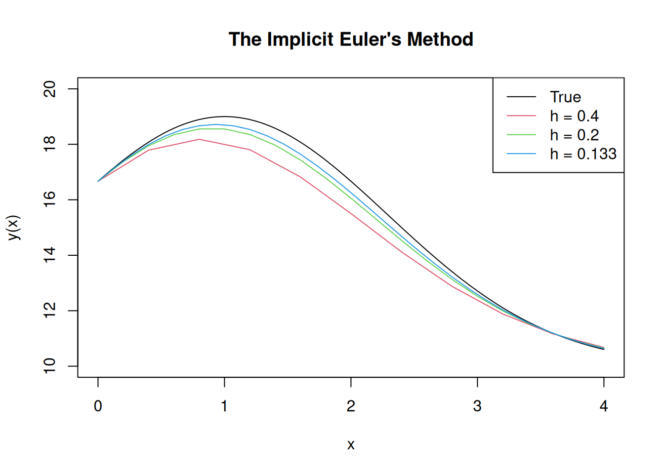
The method now undershoots the solution because it used the slope at the end points. Both methods converge linearly to the solution. In other words, the error is of order \(h\). We can to better by using better integration rules.
8.2.3 Trapezoid Rule
Lets first rewrite the result from the fundamental theorem of calculus: \[ y(x_{k+1})-y(x_k) = \int_{x_k}^{x_{k+1}} f(x,y(x)) dx. \] The right hand side can be computed by the Trapezoid method, which gives: \[ y_{k+1} = y_{k} + \frac{h}{2}\Big(f(x_{k},y_{k}) + f(x_{k+1},y_{k+1})\Big) \] It is also an implicit method that requires us to solve a nonlinear equation, but the error is of order \(h^2\) which is better than any Euler’s Methods.
myODE3 <- function(f,n,a,b,y0,from=0,to=50)
{
    h <- (b-a)/n
    f2 <- function(y,y1,x1,x,h)
        y-y1-h*(f(x,y)+f(x1,y1))/2
    x <- a+h*(0:n)
    y <- y0
    for (i in 2:(n+1))
        y[i] <- uniroot(f2,c(from,to),y1=y[i-1],
        x1=x[i-1],x=x[i],h=h)$root
    return(list(x=x,y=y,h=h))
}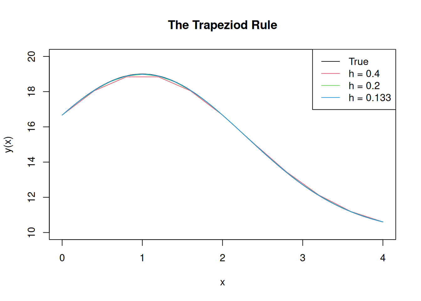
The method work nicely even for small \(h\) (\(h=.4\) corresponds to 10 points). This method, however, may not be convenient in some cases in which the nonlinear equation is hard to solve. The next method is explicit and can do even better than the Trapezoid rule.
8.2.4 Runge-Kutta Method
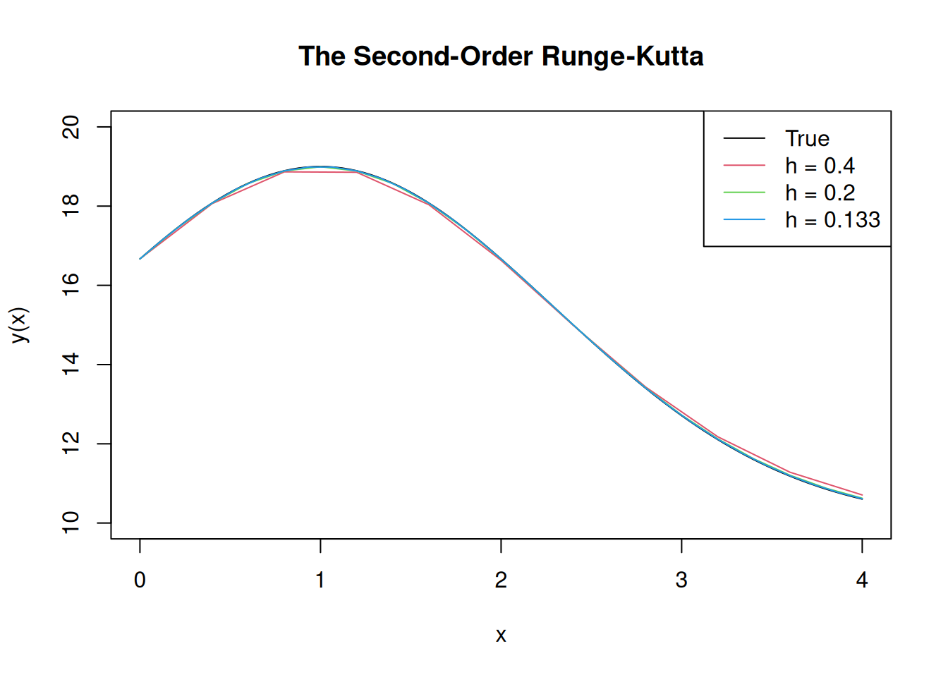
There is more than one version of this method. The idea is similar to the Trapezoid rule because it computes \(f(x,y)\) at more than one points in order to get a better approximation. The second-order Runge-Kutta (RK2) is like the Trapezoid, but the Euler’s \(Y_{k+1}\) is used instead. Its error is also \(O(h^2)\). Since it only depends on known values, we don’t need to solve a nonlinear equation: \[ y_{k+1} = y_{k} + \frac{h}{2}\Big(f(x_{k},y_{k}) + f(x_{k+1},Y_{k+1}^E)\Big), \] where \(Y_{k+1}^E=y_k+hf(x_k,y_k)\)
RK2 <- function(f,n,a,b,y0)
{
    h <- (b-a)/n
    x <- a+h*(0:n)
    y <- y0
    for (i in 2:(n+1))
        {
        YE = y[i-1] + h*f(x[i-1],y[i-1])
        y[i] <- y[i-1]+h*(f(x[i-1],y[i-1])+f(x[i],YE))/2
        }
    return(list(x=x,y=y,h=h))
}
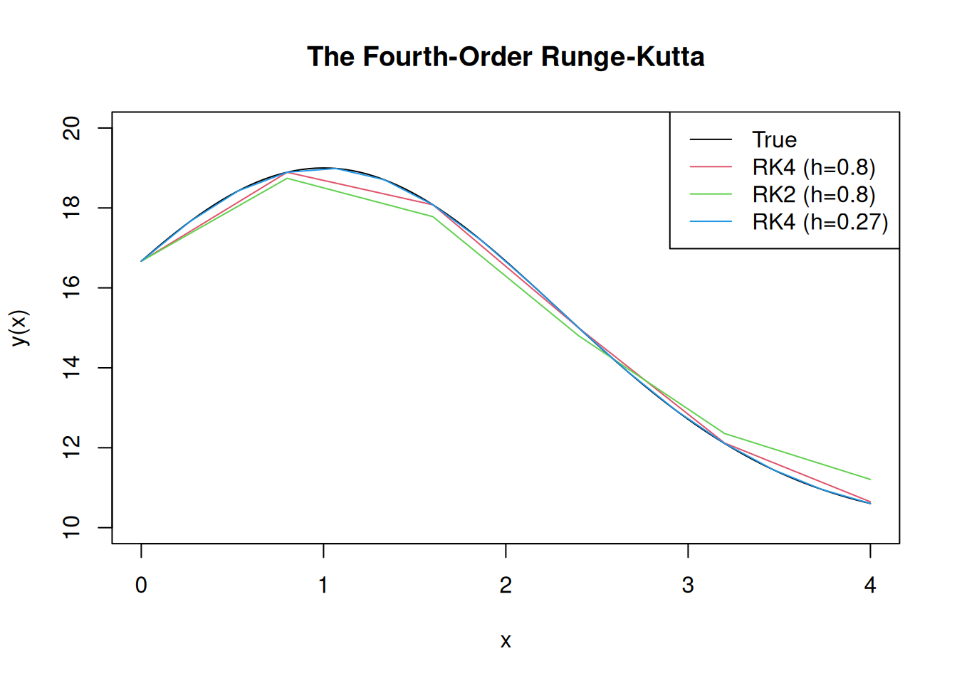
The fourth-order Runge-Kutta (RK4) evaluate \(f(x,y)\) at 4 points and its error is \(O(h^4)\)
RK4 <- function(f,n,a,b,y0)
{
    h <- (b-a)/n
    x <- a+h*(0:n)
    y <- y0
    for (i in 2:(n+1))
    {
        F1 <- f(x[i-1],y[i-1])
        F2 <- f(x[i-1]+h/2,y[i-1]+h*F1/2)
        F3 <- f(x[i-1]+h/2,y[i-1]+h*F2/2)
        F4 <- f(x[i],y[i-1]+h*F3)
        y[i] <- y[i-1]+h*(F1+2*F2+2*F3+F4)/6
    }
    return(list(x=x,y=y,h=h))
}
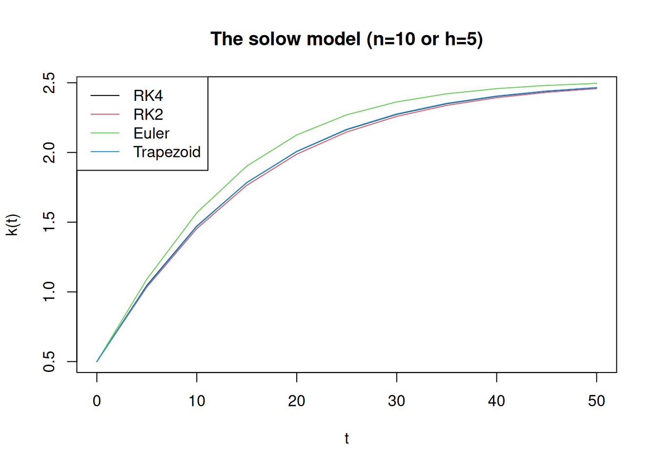
Lets now compare few methods to the Solow model. We assume the following values: \(s=0.2\), \(\delta=0.1\), \(\alpha=0.25\), and \(k(0)=0.5\).
Example 8.1 (Signaling Equilibrium) This example comes from Judd (1998), page 347. It is a simplified version of a model developed by Spence (1974). It is an initial value problem with closed form solution. We can use it to compare the performance of the different methods.
In the model, individuals of type \(n\in [n_m,n_M]\) (a measure of his ability) choose the level of education \(y\). The cost of education is \(C(y,n)\) with \(C_y>0\) and \(C_n<0\). Employers only observe \(y\) (the signal), which implies that wage, \(w(y)\), only depends on it. Individuals maximize their net income \(w(y)-C(y,n)\), which implies that \(w'(y)=C_y(y,n)\). Output produced by each individual, \(S(y,n)\), depends on his type and level of education, with \(S_y>0\), and \(S_n>0\). We assume a competitive equilibrium, which implies that \(w(y)=S(y,n)\).
Because each type will choose different level of education, we have \(y=y(n)\). To follow the book and the article, we will substitute the inverse of the optimal level of education \(n=n(y)\) in the equilibrium condition in order to obtain the differential equation. The equilibrium conditions become: \[ w'(y) = C_y(y,n(y)) \] \[ w(y) = S(y,n(y)) \] If we differentiate the second equation and substitutes the first in it, we obtain the Equation 10.4.1 of Judd: \[\begin{equation} n'(y) = \frac{C_y(y,n(y)) -S_y(y,n(y))}{S_n(y,n(y))} \tag{8.4} \end{equation}\] For the initial value, we assume that the individual with the lowest ability \(n_m\) chooses the level of education \(y_m\) that is socially optimal. It satisfies \(S_y(y_m,n_m)=C_y(y_m,n_m)\). For the numerical example, we assume that \(S(y,n)=ny^\alpha\), \(C(y,n)=y/n\), \(n_m=0.1\), \(\alpha=0.25\), and \(y_m=0.00034\). The closed form solution is given by Equation 10.4.5 of Judd. The following solves the different equation (8.4).
Spence <- function(y, alpha=0.25, nm=0.1)
{
    ym <- (nm^2*alpha)^(1/(1-alpha))
    D <- (nm/ym^(-alpha))^2*(1+alpha)/2-ym^(1+alpha)
    y^(-alpha)*sqrt(2*(y^(1+alpha)+D)/(1+alpha))
}
dN <- function(y,n, alpha=0.25)
    (1/n - alpha*n*y^(alpha-1))/y^alpha
nm <- 0.1
alpha <- 0.25
b <- 1
N <- c(5,10,20,40,100)
ym <- (nm^2*alpha)^(1/(1-alpha))
curve(Spence,ym,b,xlab="y",ylab="n(y)",main=
"Spence(74) model",n=2000)
for(i in 1:length(N))
{
s <- RK4(dN,N[i],ym,b,nm)
lines(s$x,s$y,col=(i+1)) }
l <- paste("RK4 (h=",round((b-ym)/N,3),")",sep="")
legend("bottomright",c("True",l),col=1:(length(N)+1),lty=1)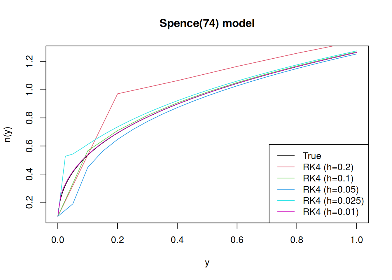
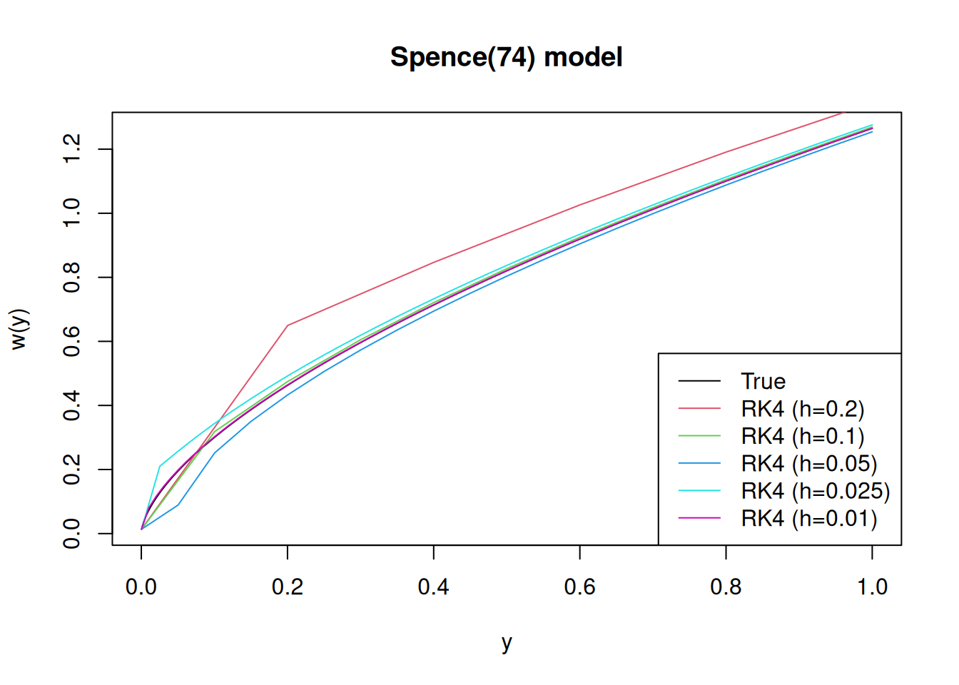
We see that the choice of \(h\) matters most when the second derivative of the solution is the highest. We can also get the solution for \(w(y)\), using the equilibrium condition.
8.3 Boundary values and the Shooting Method
Consider the life-cycle model in which consumers maximize the discounted future utility: \[ \max_c \int_0^T e^{-rt} u(c(t))dt \] subject to: \[ \dot{A} = f(A(t)) + w(t)-c(t), \] and \(A(0)=A(T)=0\). The Hamiltonian is: \[ H = u(c) + \lambda(f(A)+w-c). \] The solution implies the first order condition \[ u'(c) = \lambda \] the constraint: \[ \dot{A} = f(A(t)) + w(t)-c(t), \] and the costate equation: \[ \dot\lambda = \rho \lambda - \lambda f'(A) \] If we substitute \(\lambda\) by \(u'(c)\), and \(\dot\lambda\) by \(u''(c)\dot c\) in the last equation, we obtain the following system of differential equations: \[\begin{equation} \begin{split} \dot{A} = & f(A) + w-c\\ \dot c = & \frac{u'(c)}{u''(c)}(\rho-f'(A)) \end{split} \tag{8.5} \end{equation}\] with initial value \(A(0)=0\), and boundary condition \(A(T)=0\).
This kind of problems is quite different from initial value problems because we need to restrict the last value without knowing the solution. The Shooting method is a trial-and-error approach. In the above problem, \(A(T)\), given \(A(0)=0\), depends of the initial values \(c(0)\). The method consists in guessing \(c(0)\), and modifying it until \(A(T)\) is sufficiently close to 0.
First, we need to adapt the RK4() function for system of equations. In the following, \(f\) is a function \((x,y)\) which returns an \(n\times 1\) vector, \(x\in [a,b]\), and \(y\in \mathbb{R} ^n\).
RK4 <- function(f,n,a,b,y0,...)
{
    h <- (b-a)/n
    x <- a+h*(0:n)
    y <- matrix(y0,nrow=1)
    for (i in 2:(n+1))
    {
        F1 <- f(x[i-1],y[i-1,],...)
        F2 <- f(x[i-1]+h/2,y[i-1,]+h*F1/2,...)
        F3 <- f(x[i-1]+h/2,y[i-1,]+h*F2/2,...)
        F4 <- f(x[i],y[i-1,]+h*F3,...)
        yi <- y[i-1,]+h*(F1+2*F2+2*F3+F4)/6
        y <- rbind(y,yi)
    }
    return(list(x=x,y=y,h=h))
}
For the numerical exercise, we assume that \(u(c)=c^{1+\gamma}/(1+\gamma)\), \(w(t)=1\) if \(M\leq t \leq R\) and 0 otherwise, \(\rho=0.04\), \(f(A)=rA\) with \(r=0.10\), \(\gamma=-0.5\), \(T=55\), \(M=10\), and \(R=40\). The following function returns the right hand side of the system (8.5), with \(y=\{c,A\}'\):
LifeCycle <- function(x,y,rho=0.04,r=0.10,gamma=-2,M=10,R=40)
{
    w <- (x<=R)*(x>=M)
    y1 <- r*y[2]+w-y[1]
    y2 <- (rho-r)*y[1]/gamma
    c(y2,y1)
}
Lets first start with \(c(0)=0.3\), and \(c(0)=0.2\):
h <- .01
c0 <- c(.2,.3)
n <- floor(55/h)
s <- RK4(LifeCycle,n,0,55,c(c0[1],0))
s2 <- RK4(LifeCycle,n,0,55,c(c0[2],0))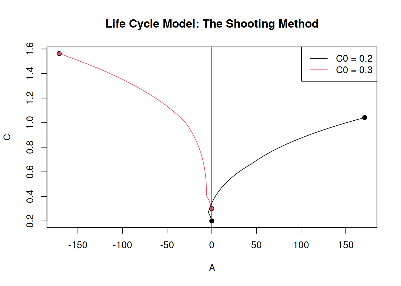
The end point of the solution path should be 0. For \(c(0)=0.2\), \(A(55)>0\), and for \(c(0)=0.3\), \(A<0\). The find the right \(c(0)\) we can use a bisection method. The following is a function that can be used in the Bisection function of Chapter 5:
f <- function(c0)
{
    n <- floor(55/0.01)
    s <- RK4(LifeCycle,n,0,55,c(c0,0))
    return(s$y[n+1,2])
}
res <- Bisection(f,.2,.3)
res
##
## Method: Bisection
## Message: Converged after 20 iterations
##
## The solution is: 0.2500609 , and f(x) is 3.074027e-05
## Precision: 9.536743e-08We can then use that value to plot the solution.
s <- RK4(LifeCycle,n,0,55,c(res$sol,0))
plot(s$y[,2],s$y[,1],type="l",xlab="A",ylab="C",
main="Life Cycle Model: The solution")
abline(v=0)
points(c(0,0),c(res$sol,s$y[n+1,1]),pch=c(21,21),bg=c(1,1))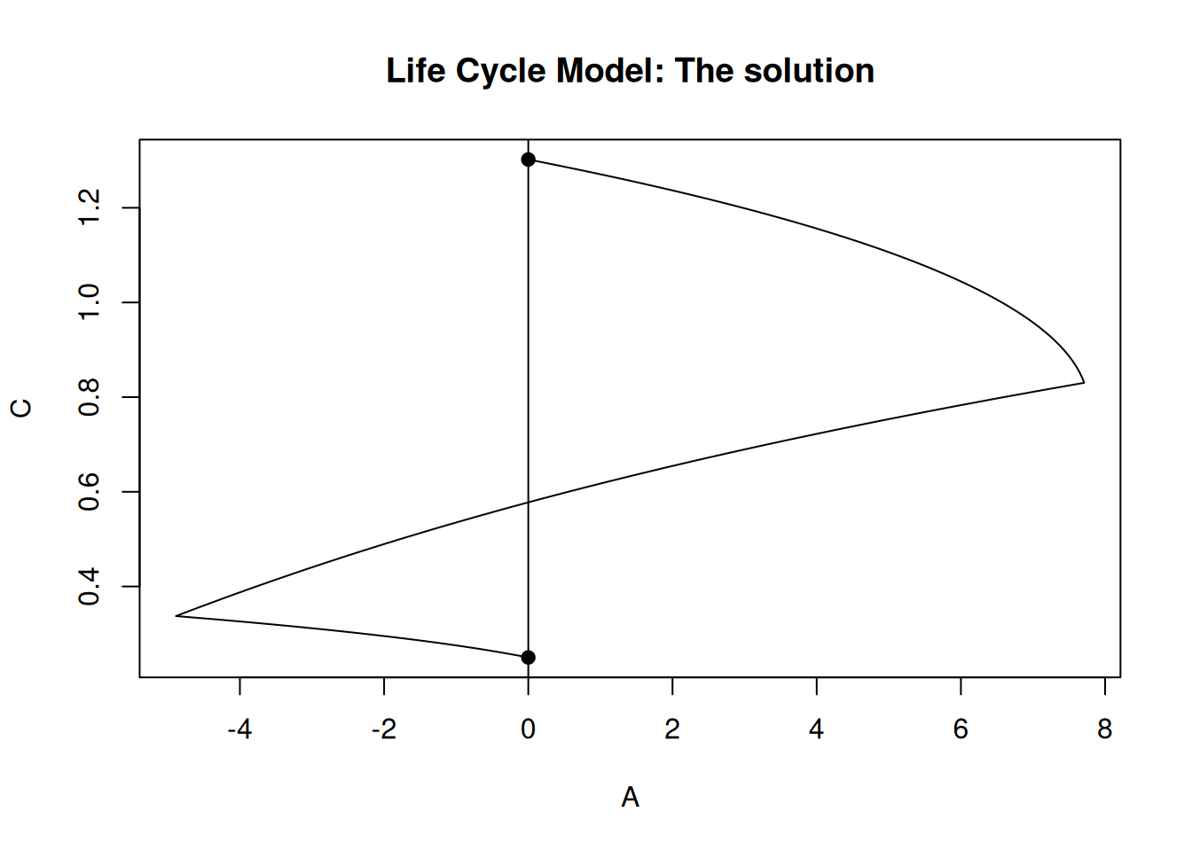
8.3.1 Infinite Horizon Models
Consider the following model: \[ \max_c\int_0^\infty e^{-\rho t} u(c) dt \] subject to \(\dot{k}=f(k)-c\), and \(k(0)=k_0\). We don’t have explicit boundary conditions, but we have to assume that \(\lim_{t\rightarrow \infty} |k(t)| < \infty\) (which also implies the convergence of \(|c(t)|\)). We know for the above model that the only possible path is the one that will make \(k(t)\) and \(c(t)\) converge to their respective steady state values, \(k^*\) and \(c^*\). The first method is to forward shooting and it consists in choosing the path that leads as close as possible to the steady state. The following algorithm is the one proposed on page 357 of Judd, and it is for the case in which \(k_0<k^*\). We also use the specification given on page 359.
growth <- function(x,y)
{
    y1 <- -(.05-0.05*y[2]^(-.75))*y[1]/2
    y2 <- 0.2*y[2]^0.25-y[1]
    c(y1,y2)
}
RK4G <- function(f,h,y0,maxit=1000)
{
    #The difference: it stops when either df/dy<0
    x <- 0
    y <- matrix(y0,nrow=1)
    i <- 1
    while(TRUE)
    {
        F1 <- f(x[i],y[i,])
        F2 <- f(x[i]+h/2,y[i,]+h*F1/2)
        F3 <- f(x[i]+h/2,y[i,]+h*F2/2)
        F4 <- f(x[i]+h,y[i,]+h*F3)
        y1 <- y[i,]+h*(F1+2*F2+2*F3+F4)/6
        x <-  c(x,x[i]+h)
        y <- rbind(y,y1)
        if (any(f(x[i+1],y1)<0))
            break
        if (i>maxit){
            warning("maxit reached")
            break}
        i <- i+1
    }
    return(list(T=i,y=y,x=x))
}
fShooting <- function(f,k0,h=0.01,eps=1e-7,maxit=20)
{
    cL <- 0; cH <- 0.2*k0^0.25
    cSteady <- 0.2; i <- 1
    while(TRUE)
        {
        c0 <- (cL+cH)/2
        res <- RK4G(f,h,c(c0,k0),maxit=2000)
        T <- res$T+1
        if (abs(res$y[T,1]-cSteady)<eps)
            break
        if (i>maxit){
            warning("Maxit reached")
            break}
        ydot <- f(res$x[T],res$y[T,])
        if (ydot[1]<0)
            cL <- c0
        else
            cH <- c0
        i <- i+1
        }
    return(res)
}
res <- fShooting(growth,.2,eps=1e-3,maxit=1000,h=.1)
k <- res$y[,2]
c <- res$y[,1]
curve(.2*x^.25,0,1.50,xlab="K(t)",ylab="C(t)",n=1000,xlim=c(-.2,1.8),
main="Infinite-Horizon problem with Forward Shooting",lwd=2)
abline(v=1,lwd=2,col=2)
text(1.075,.02,expression(dot(C)==0),col=2)
text(1.6,.22,expression(dot(K)==0),col=1)
lines(k,c,col=4,lwd=4)
text(k[20],c[20],"Stable Path",col=4,pos=4)
points(k[1],c[1],pch=21,bg=4)
text(k[1]+.05,c[1],paste("(",round(k[1],3),", ",round(c[1],4),")",sep=""),pos=1,col=4)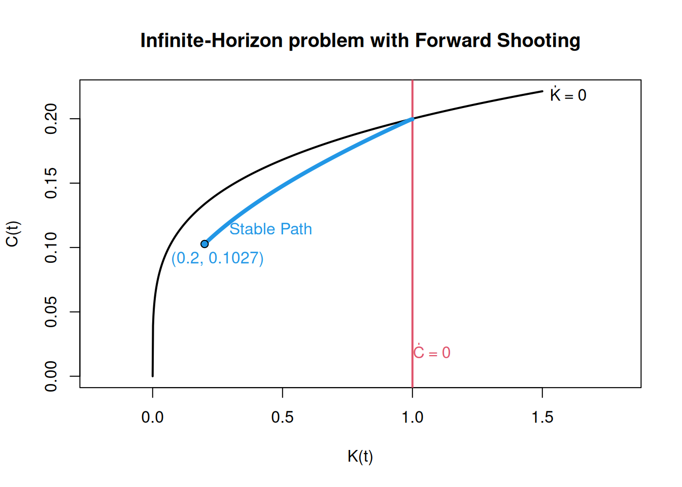
This method is time consuming and hard to perform because a slight deviation from the stable path leads to the unstable one. Another way is to do the reverse shooting on \(-f(x,y)\). The idea is to transform the stable path into the unstable one. From the phase diagram, a small deviation from the steady state leads to the unstable path. We can therefore use that property to generate the solution.
revGrowth <- function(x,y)
{
    y1 <- -(.05-0.05*y[2]^(-.75))*y[1]/2
    y2 <- 0.2*y[2]^0.25-y[1]
    -c(y1,y2)
}
res1 <- RK4(revGrowth,1000,0,300,c(.2,1.01))
res2 <- RK4(revGrowth,1000,0,300,c(.2,.99))
curve(.2*x^.25,0,1.50,xlab="K(t)",ylab="C(t)",n=1000,xlim=c(-.2,2),ylim=c(0,.4),
main="Infinite-Horizon problem with Reverse Shooting",lwd=2)
abline(v=1,lwd=2,col=2)
text(1.075,.02,expression(dot(C)==0),col=2)
text(1.6,.22,expression(dot(K)==0),col=1)
# differential equations (ODE), partial differential equations
points(k[1],c[1],pch=21,bg=4)
text(k[1]+.05,c[1],paste("(",round(k[1],3),", ",round(c[1],4),")",sep=""),pos=1,col=4)
lines(res1$y[,2],res1$y[,1],col=3,lwd=2)
lines(res2$y[,2],res2$y[,1],col=3,lwd=2)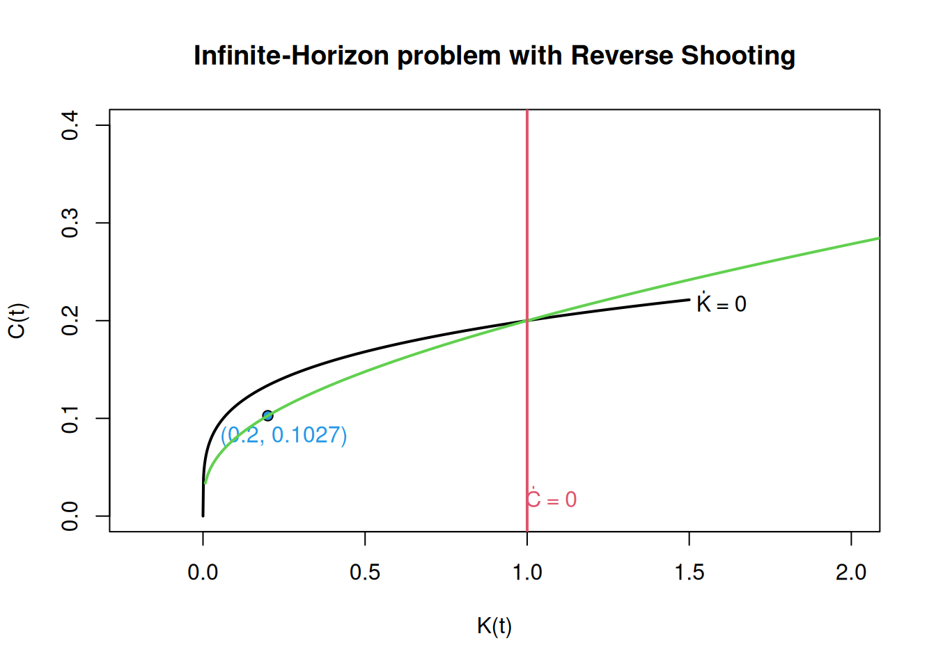
We could then use those points to obtain \(c(0)\) for different \(k(0)\). The interpolation method is a nice way to do it:
##         x         y
## 0.2000000 0.1027205## x y
## 0.5000000 0.1477963## x y
## 1.5000000 0.2417928Another way to apply the reverse shooting method is to solve directly for the stable path \(c(t) = C(k(t))\). If we differentiate the identity, we get \(C'(k) = \dot{c}/\dot{k}\), starting at the steady states \(C(K^*) = c^*\), which implies: \[\begin{equation} C'(k) = \frac{u'(C)}{u''(C)}\frac{\rho-f'(k)}{f(k)-C} \tag{8.6} \end{equation}\] with \(C'(k^*)\) given by Equation 10.7.7 of Judd (1998).
Exercise 8.1 Replicate Table 10.2 of Judd (1998), using the reverse shooting method applied to the differential equation (8.6)
Exercise 8.2 Answer Exercises 2, 5, and 6 of Judd (1998) (Chapter 10)
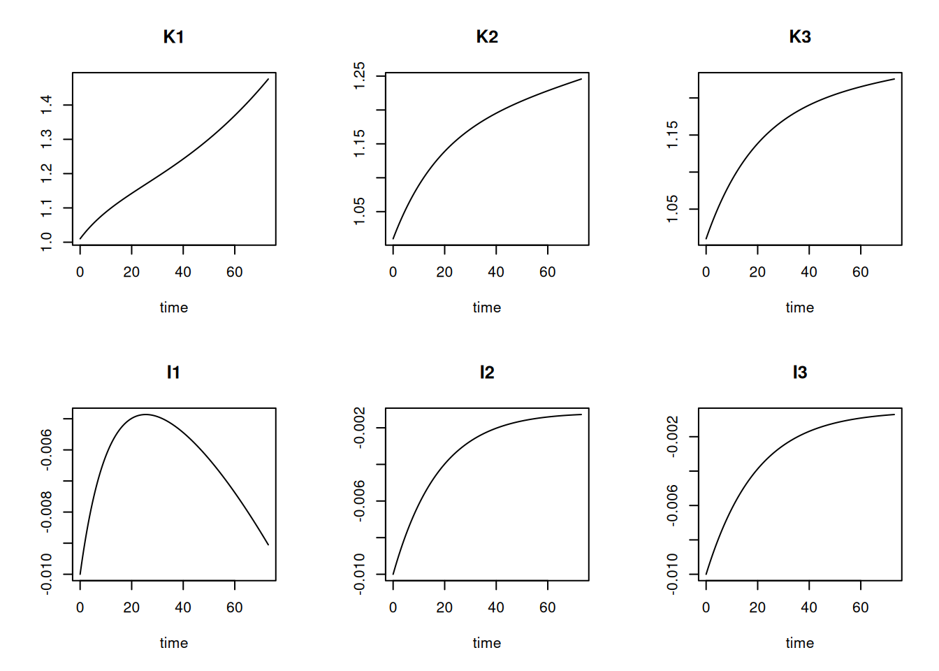
Example 8.2 (A Multidimentional Problems) We conclude the section with an example of reverse shooting for multidimensional problems. We consider the growth model with 3 sectors presented in exercise 7, with \(u(c)=\log(c)\), \(\rho=0.05\), \(\alpha_1=0.25\), \(\alpha_2=0.35\), \(\alpha_3=0.4\), \(\gamma_1=10\), \(\gamma_2=50\), \(\gamma_3=100\), and \(k_i(0) = 0.5\) for \(i=1,2,3\). First, we need to compute the steady state. I don’t want to compute it manually, so I will use a method from Chapter 5. First, the solution implies the following differential equations. \[ \dot{\lambda}_i = \rho\lambda_i - \frac{\rho k_i^{\alpha_i-1}}{C}, \] \[ \dot{k}_i = I_i, \] for \(i=1,2,3\) with \[ \lambda_i = \frac{1+2\gamma_i I_i}{C} \] and \[ C = \rho \left(\frac{k_1^{\alpha_1}}{\alpha_1}+\frac{k_2^{\alpha_2}}{\alpha_2}+\frac{k_3^{\alpha_3}}{\alpha_3}\right) -\left(I_1+I_2+I_3+\gamma_1I_1^2+\gamma_2I_2^2+\gamma_3I_3^2\right) \] The steady state values are \(k_i^*=1\), \(I_i^*=0\), and \(\lambda_i^*=1/C\). There is two approaches to solve the problem. First, we can follow the procedure on page 361 of Judd, and solve for \(I_i(t)\) using the maximum principle (the first order conditions), and substitute the solution into the differential equations. However, there is no closed form solution \(I_i(t)\). We can solve it using a nonlinear solver but it may be unstable because there are multiple solutions. The following follows that method:
MGrowth <- function(x,y)
    {
    alpha <- c(.25,.35,.4)
    rho = .05
    gamma = c(10,50,100)
    I0 <- c(0,0,0)
    I <- function(I,K,Lambda){
        C <- sum(rho*K^alpha/alpha)-sum(I)-sum(gamma*I^2)
        C*Lambda-1-2*gamma*I
        }
    Iv <- Broyden(I,I0,K=y[1:3],Lambda=y[4:6])$sol
    C <- sum(rho*y[1:3]^alpha/alpha)-sum(Iv)-sum(gamma*Iv^2)
    dy2 <- rho*y[4:6]-rho*y[1:3]^(alpha-1)/C
    return(-c(Iv,dy2))
    }
SteadyC <- sum(rho/alpha)
SteadyK <- c(1,1,1)
SteadyL <- rep(1/SteadyC,3)
y <- c(SteadyK*1.001,SteadyL)
res1 <- RK4(MGrowth, n, 0, T, y)I am not showing the result because it is not satisfying. In the second method, I substitute the \(\lambda_i\) and \(\dot{\lambda}_i\) by \(I_i\) and \(\dot{I}_i\). We replace \(\lambda_i\) by \[ \lambda_i = \frac{1+2\gamma_i I_i}{C} \] and \(\dot{\lambda}_i\) by \[ \dot{\lambda}_i = -\frac{1+2\gamma_i I_i}{C^2}\dot{C} + \frac{2\gamma_i\dot{I}_i}{C} \] Because \(dot{C}\) depends on all \(\dot{k}_i\) and \(\dot{I}_i\), we need to solve a linear system of equations to obtain the 6 differential equations.
MGrowth2 <- function(x,y)
{
    alpha <- c(.25,.35,.4)
    rho = .05
    gamma = c(10,50,100)
    K <- y[1:3]
    I <- y[4:6]
    C <- sum(rho*y[1:3]^alpha/alpha)-sum(I)-sum(gamma*I^2)
    Ai <- -1/C^2*(1+2*gamma*I)
    Bi <- 2*gamma/C
    Ei <- rho*(1+2*gamma*I)/C-rho*K^(alpha-1)/C
    A <- c(rho*K^(alpha-1), -(1+2*gamma*I))
    W <- Ai%o%A
    diag(W[1:3,4:6]) <- diag(W[1:3,4:6]) + Bi
    W <- rbind(W,cbind(diag(3),0,0,0))
    -solve(W,c(Ei,I))
}
T <- 73
n <- 400
SteadyK <- c(1,1,1)
y <- c(SteadyK*1.01,rep(-0.01,3))
res <- RK4(MGrowth2, n, 0, T, y)
y <- c(SteadyK*.99,rep(0.01,3))
res1 <- RK4(MGrowth2, n, 0, T, y)
Y <- rbind(c(SteadyK,0,0,0),res$y)
Y <- rbind(res1$y[(n+1):1,],Y)
plot(Y[,1],Y[,4],type="l",main="Multifactor Growth Model",
xlab=expression(K[1](t)),ylab=expression(I[1](t)))
points(SteadyK[1],0,pch=21,bg=1)
text(SteadyK[1],0,"Steady state",bg=1,pos=1)
Y <- rbind(c(SteadyK,0,0,0),res$y[-(1:(n/2)),])
Y <- rbind(res1$y[(n+1):(n/2+1),],Y)
lines(Y[,1],Y[,4],col=4,lty=2,lwd=2)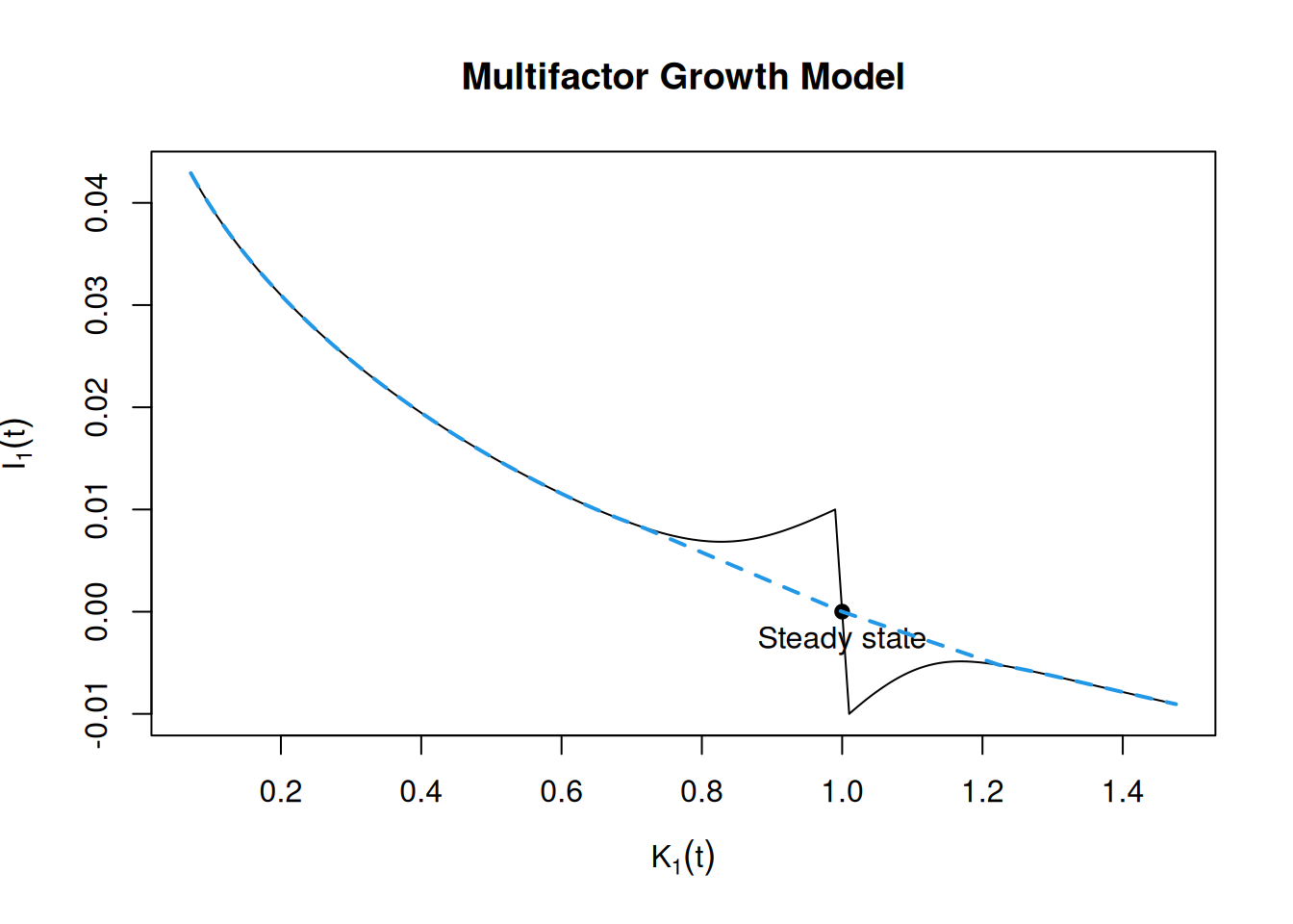
Y <- rbind(c(SteadyK,0,0,0),res$y)
Y <- rbind(res1$y[(n+1):1,],Y)
plot(Y[,2],Y[,5],type="l",main="Multifactor Growth Model",
    xlab=expression(K[2](t)),ylab=expression(I[2](t)))
points(SteadyK[1],0,pch=21,bg=1)
text(SteadyK[1],0,"Steady state",bg=1,pos=1)
Y <- rbind(c(SteadyK,0,0,0),res$y[-(1:(n/2)),])
Y <- rbind(res1$y[(n+1):(n/2+1),],Y)
lines(Y[,2],Y[,5],col=4,lty=2,lwd=2)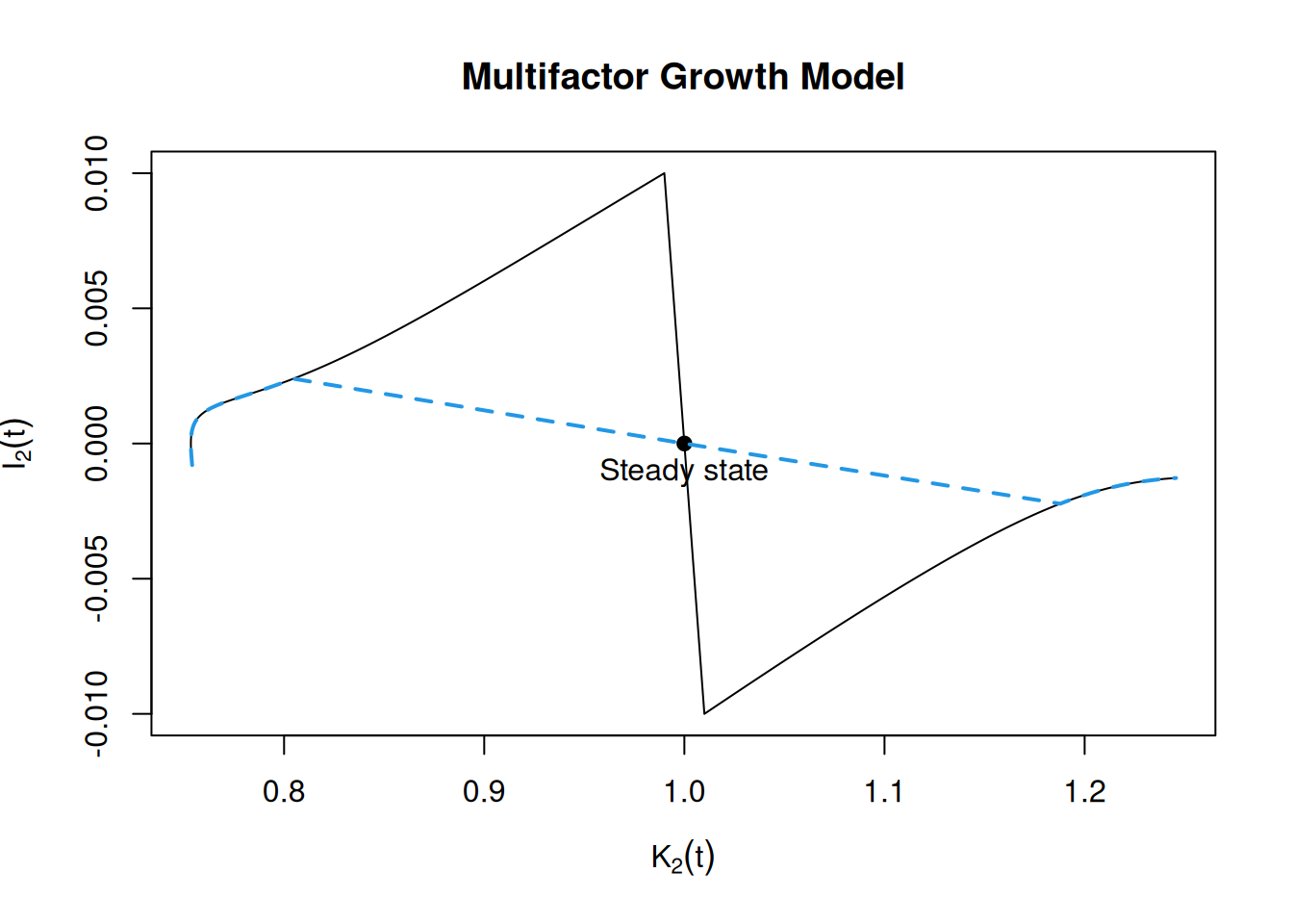
8.4 Projection Methods (incomplete)
For now, I just give the idea behind the projection method. We don’t have time this semester to go into more details. Suppose we want to solve \(y'(t)=f(t,y)\) with \(y(0)=y_0\). The idea is to approximate the \(y(t)\) by another function \(\phi(t)\) with the property \(\phi(0)=y_0\), for an initial value problem, and \(\phi(T)=y_T\), for a boundary value problem. Consider the example given on page 370 of Judd, \(y'(t) = y(x)\), with \(t\in[0,3]\), and \(y(0)=1\). The solution is \(e^t\). Consider the following approximation: \[ \phi(t; a) = 1 + \sum_{i=1}^n a_i t^i \] then, the differential equation implies: \[ \sum_{i=1}^n i a_i t^{i-1} \approx 1 + \sum_{i=1}^n a_i t^i \] or \[ R(x; a) = -1 + \sum_{i=1}^n a_i (it^{i-1}-t^i) \approx 0, \] where \(R(x;a)\) is called the residual function. We want to choose \(a\) in such a way that \(R(x;a)\) is as close to 0 as possible for all \(x\). The simpler approach is to use the least square method, and minimize \(\int_0^3 R(x;a)dx\). Suppose \(n=3, 4\), then:
R_LS <- function(a,from,to)
{
    Rfct <- function(x)
  {
        n <- length(a)
        R <- -1
        for (i in 1:n)
            R <- R+a[i]*(i*x^(i-1)-x^i)
        return(R^2)
    }
    integrate(Rfct,from,to)$value
}
We can get the coefficients \(a_i\)’s by minimizing R\_LS (notice that the solution can be obtained by solving a linear system of equations).
## [1] 1.2903209 -0.8064510 0.6586022f <- function(x)
apply(as.matrix(x),1,function(x) 1+sum(res$par*x^(1:length(res$par))))
Q <- curve(f,0,3,main="Polynomial approximation of Y(t) in Y'-Y=0")
res <- optim(c(0,0,0,0),R_LS,from=0,to=3,method="BFGS")
res$par## [1] 0.7701986 1.1310133 -0.3906775 0.2090132lines(Q$x,f(Q$x),col=2)
lines(Q$x,exp(Q$x),col=3)
legend("topleft",c("Estimated (n=3)", "Estimated (n=4)", "True"),col=1:3,lty=1)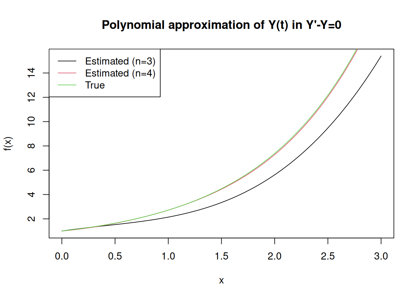
The Subdomain method finds the \(n\) \(a_i\)’s that satisfy \(\int_{D_i} R(x;a)=0\) for the \(n\) intervals \(D_i\).
R_SD <- function(a,from,to,D)
{
    Rfct <- function(x)
    {
        n <- length(a)
        R <- -1
        for (i in 1:n)
            R <- R+a[i]*(i*x^(i-1)-x^i)
        return(R)
    }
    from <- seq(from,to,length=(D+1))
    r <- sapply(1:D,function(i) integrate(Rfct,from[i],from[i+1])$value)
}
R_Galerkin <- function(a,from,to)
{
    Rfct <- function(x, which)
    {
        n <- length(a)
        R <- -1
        for (i in 1:n)
            R <- R+a[i]*(i*x^(i-1)-x^i)
        return(R*x^which)
    }
    r <- vector()
    for (i in 1:length(a))
        r <- c(r,integrate(Rfct,from,to, which=i)$value)
    return(c(r))
}
res <- Broyden(R_SD,c(0,0,0),from=0,to=3,D=3)
res$sol # see table 11.1 of Judd
## [1] 2.5 -1.5 1.0## [1] 2.5 -1.5 1.0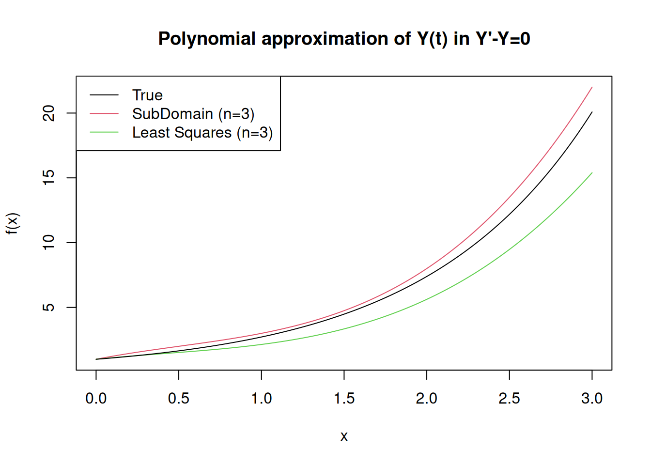
The method of collocation sets \(R(x_i,a)=0\) for \(n\) points \(x_i\). The Uniform Collocation set the points uniformly between [0,3], and the Chebyshev Collocation is based on the Chebyshev nodes.
CollCheby <- function()
{
    x <- 3/2*c(cos(5*pi/6)+1,1,cos(pi/6)+1)
    A <- vector()
    for (i in 1:3)
    {
        w <- (1:3)*x[i]^(0:2)-x[i]^(1:3)
        A <- rbind(A,w)
    }
    return(solve(A,rep(1,3)))
}
a <- CollCheby()
a
## [1] 1.6923077 -1.2307692 0.8205128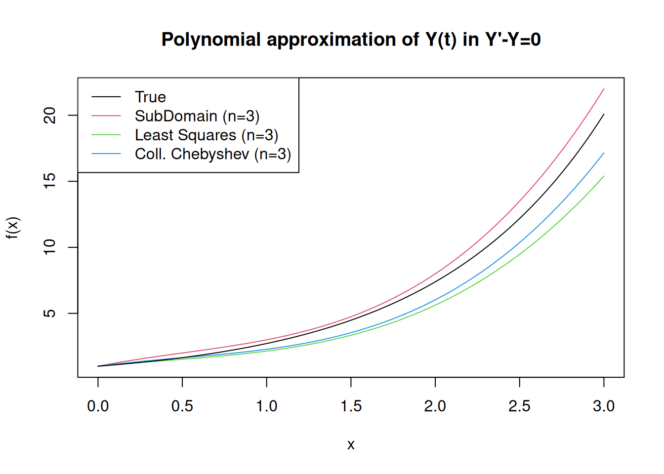
Exercise 8.3 Reproduce Table 11.2 of Judd (1998)
I conclude the section with the life cycle model. The following functions solve the problem using the Chebyshev polynomial and the Collocation method for obtaining the coefficients (The function are written for \(t\in[a,b]\) with \(A(a)=A(b)=0\) as boundary condition. Also, we assume that \(w(t)=0.5+t/10-4(t/50)^2\), and \(u(c)=c^{\gamma+1}/{\gamma+1}\) (see page 389 of Judd):
Cheby <- function(t,i,a,b)
    cos(i*acos(2*t/(b-a) - 1))
DCheby <- function(t,i,a,b)
    sin(i * acos(2 * t/(b - a) - 1)) * (i * (2/(b - a)/sqrt(1 - (2 * t/(b - a) - 1)^2)))
A <- function(t, aVec, a, b)
{
    # a[1] = a_0 and a[n] = a_(n-1)
    # valid for c as well
    n <- length(aVec)
    A <- rep(0,length(t))
    for (i in 1:n)
        A <- A+aVec[i]*Cheby(t,(i-1),a,b)
    A
}
Adot <- function(t, aVec, a, b)
{
    # a[1] = a_0 and a[n] = a_(n-1)
    # valid for c as well
    n <- length(aVec)
    A <- rep(0,length(t))
    for (i in 1:n)
        A <- A+aVec[i]*DCheby(t,(i-1),a,b)
    A
}
getSol <- function(n, a, b)
{
    w <- function(t)
        0.5+t/10-4*(t/50)^2
    t <- gauss.quad(n-1,kind="chebyshev1")$node*(b-a)/2+(b-a)/2
    f <- function(theta)
    {
        aVec <- theta[1:n]
        cVec <- theta[(n+1):(2*n)]
        R1 <- Adot(t, cVec, a, b)-0.025*A(t,cVec,a,b)
        R2 <- Adot(t,aVec,a,b) - 0.1*A(t,aVec,a,b)-w(t)+A(t,cVec,a,b)
        R3 <- A(a,aVec,a,b)
        R4 <- A(b,aVec,a,b)
        c(R1,R2,R3,R4)
    }
    res <- Broyden(f,rep(0,2*n),maxit=300,eps=1e-9)
    t <- seq(a,b,length=200)
    At <- A(t,res$sol[1:n],a,b)
    Ct <- A(t,res$sol[(n+1):(2*n)],a,b)
    list(Coef = res, At = At, Ct = Ct, t = t)
}library(statmod)
res <- getSol(10,0,50)
plot(res$Ct,res$At,type="l",main="Life Cycle: Projection method",
ylab="A(t)",xlab="C(t)")
points(res$Ct[c(1,length(res$t))],res$At[c(1,length(res$t))],
pch=21,bg=1)
abline(h=0)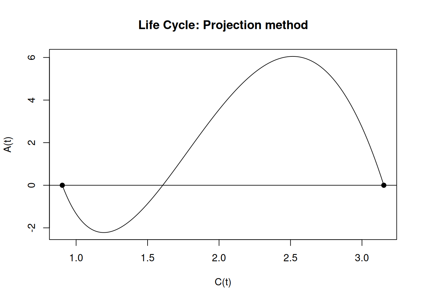
See how fast is it compare to the shooting method.
Exercise 8.4 Solve the growth model on page 392 of Judd. You must obtain \(C(k)\) directly by approximating \(C(k)\) using Chebyshev polynomials and the Collocation Method.
8.5 Partial Differential Equation: The Heat Equation
Let \(\theta(x,t)\) be a function that returns the temperature of a metal bar at time \(t\in[0,\infty]\), and location \(x\). If we suppose that the length of the bar is 1, then \(x\in[0,1]\), where 0 and 1 are the two extremities. The partial differential equation that represents how temperature is distributed along the bar is: \[ \theta_t - \theta_{xx} = 0 \] In the standard heat equation, we assume that something cool down the temperature at both extremities. We therefore have the boundary condition \(\theta(0,t)=\theta(1,t)=0\). It says that the change of temperature is proportional to the speed at which temperature moves from one point to another on the bar. Why would an economist cares about the heat equation? In some applications, the differential equation can be written as the heat equation. It is the case of the problem required to derive the Black and Scholes formula.
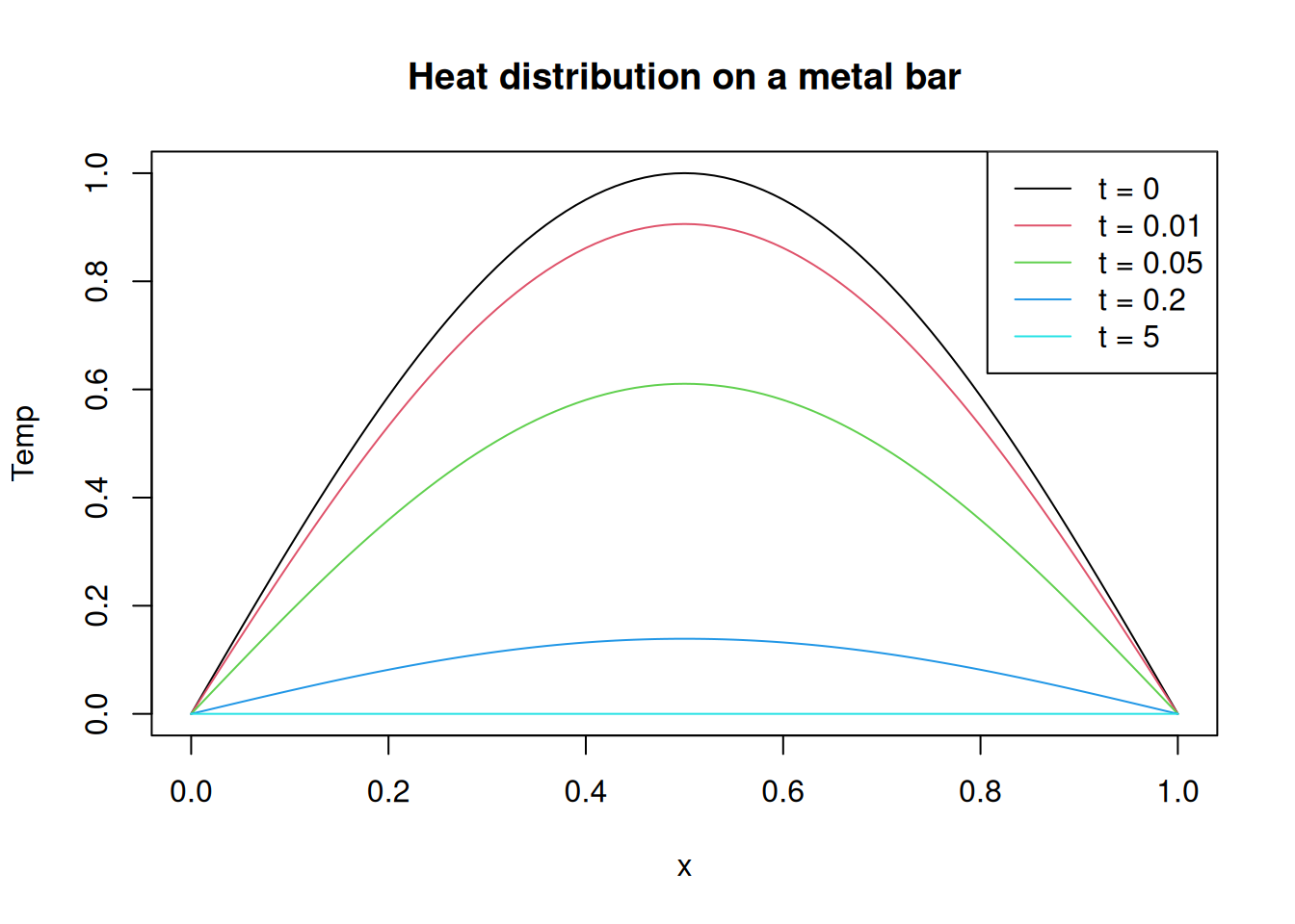
If we assume that \(\theta(x,0)=\sin(\pi x)\), the solution is \(\theta(x,t) = e^{-\pi^2t}\sin(\pi x)\).
For a given \(t\), we can use the following approximation: \[ \theta(x,t)\approx \hat{\theta}(x,t)=\sin(\pi x) + \sum_{i=1}^n a_i(t)(x-x^i) \] The approximation satisfies the condition \(\theta(x,0)=\sin(\pi x)\) if \(a_i(0)=0\). By construction, the condition \(\theta(0,t)=\theta(1,t)=0\) is satisfied. The unknown coefficients are functions of \(t\). If we apply the heat equation to the approximation, and use projection conditions, we obtain a differential equation for \(a_i(t)\) with the initial conditions \(a_i(0)=0\). We can use any method to solve initial value problems or use another projection method. Let, for example, \(t\in[0,1]\). Since we need \(a_i(0)=0\), we can approximate the functions by: \[ a_i(t) = \sum_{j=1}^m a_{ij} t^j, \] which gives: \[ \hat{\theta}(x,t)=\sin(\pi x) + \sum_{i=1}^n\sum_{j=2}^m a_{ij}(x-x^i)t^j \] The projection methods consists in computing the residual function \(R(x,t,a)\) and use conditions such as Chebyshev-Collocation or Galerkin to obtain the \(a_{ij}\). We can show that for all cases, the problem can be written as a system of \((n-1)m\) linear equations \(Ba=c\). The problem is to find the right method and the right basis functions so that the linear system if well-conditioned. We will instead solve it using finite difference (see Golub and Ortega (1992)).
Let \(\theta_i^k=\theta(x_i,t_k)\), with \(i=0,...,n+1\), and \(k=0,...,m\) , then we can write the Heat equation using finite difference as (I use the implicit Euler method because of its stability, as shown bellow): \[ \frac{\theta_i^{k+1} -\theta_i^{k}}{h_t} = \frac{\theta_{i+1}^{k+1}-2\theta_i^{k+1}+\theta_{i-1}^{k+1}}{h_x^2}, \] where \(h_x=\Delta x\), and \(h_t=\Delta t\). The boundary conditions imply that \(\theta_0^k=\theta_{n+1}^k=0\) \(\forall~k\), and \(\theta_i^0=\sin(\pi x_i)\). If we define \(\mu\) as \(h_t/h_x^2\), we can write the algorithm as: \[ \begin{pmatrix} 1+2\mu & -\mu & 0 & 0 &\cdots & 0\\ -\mu & 1+2\mu & -\mu & 0 & \cdots & 0\\ 0 & \ddots & \ddots & \ddots & \ddots & \vdots\\ \vdots&\ddots&\ddots&\ddots&\ddots&0\\ 0 & \cdots & 0 &-\mu & 1+2\mu & -\mu \\ 0 & \cdots & 0 & 0 & -\mu & 1+2\mu\\ \end{pmatrix} \theta^{k+1} = \theta^{k}, \] where \(\theta^k=\{\theta_1^k,...,\theta_n^k\}'\). The transition matrix \(A\) is tridiagonal, which makes the system easy to solve, and is diagonally dominant. Also, its eigenvalues are all strictly greater than 1 which implies that the eigenvalues of \(A^{-1}\) are strictly less than one. The iterative procedure is therefore convergent. To see that, we can write \(A\) as \(I+\mu B\), where \(B\) is also tridiagonal, with \(B_{ii}=2\) and \(B_{i,i+1}=B_{i,i-1}=-1\). We can show that the \(i^{th}\) eigenvalue of \(B\) is \(2[1+\cos(i\pi/(n+1))]\). The \(i^{th}\) eigenvalue of \(A\) is therefore \(1+2\mu[1+\cos(i\pi/(n+1))]>1\). The explicit Euler method does not possess this property. The following function computes the solution using this method:
Heat1 <- function(n,m, x=NULL, t=NULL)
{
    # Implicit Euler
    if(is.null(t))
        t <- seq(0,1,len=m)
    else
        m <- length(t)
    if(is.null(x))
        x <- seq(0,1,len=n+2)
    else
        n <- length(x)-2
    a <- (t[2]-t[1])/(x[2]-x[1])^2
    A <- matrix(0,n,n)
    diag(A) <- 1+2*a
    diag(A[-1,-n]) <- -a
    diag(A[-n,-1]) <- -a
    theta <- matrix(sin(pi*x[-c(1,n+2)]),ncol=1)
    for (i in 2:m)
        theta <- cbind(theta,solve(A,theta[,(i-1)]))
    return(list(Theta=rbind(0,theta,0),t=t,x=x))
}
We can then solve the problem quickly for all \(t_k\in[0,1]\) and \(x_i\in[0,1]\):
library(lattice)
res <- Heat1(50,50)
p <- expand.grid(res$x,res$t[1:20])
t <- p$Var2
x <- p$Var1
theta <- res$Theta
wireframe(c(theta[,1:20])~t*x,zlab=expression(theta(x,t)),main="Solution of the Heat Equation",
     scales = list(arrows = FALSE),
     drape = TRUE, colorkey = TRUE)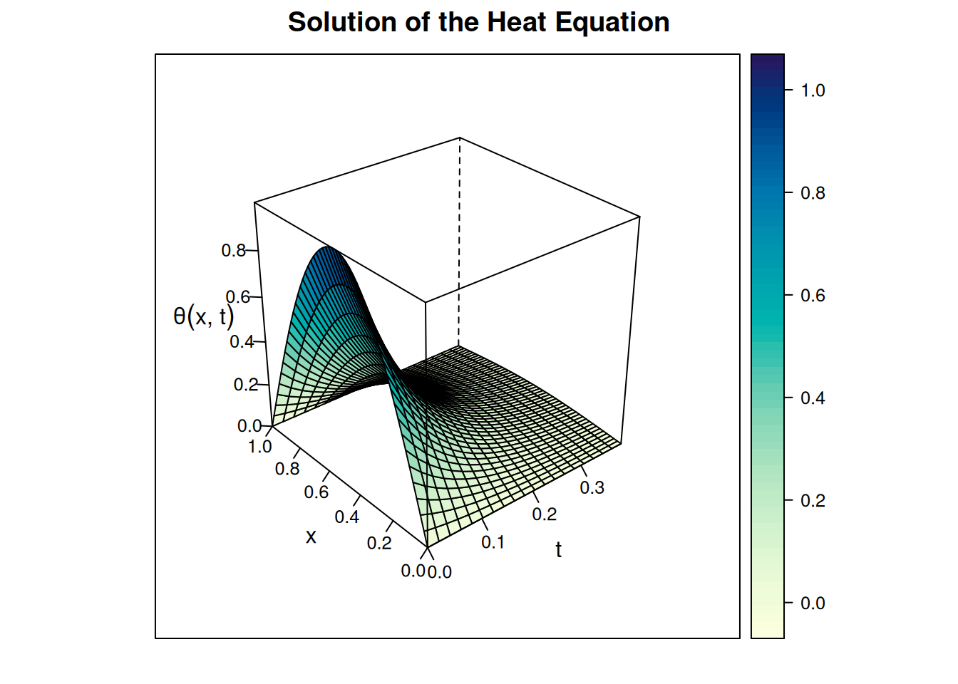
Before comparing the method with the true solution, we will look at an improve version of the above method. We can use the trapezoid rule: \[ \frac{\theta_i^{k+1} -\theta_i^{k}}{h_t} = \frac{\theta_{i+1}^{k}-2\theta_i^{k}+\theta_{i-1}^{k} + \theta_{i+1}^{k+1}-2\theta_i^{k+1}+\theta_{i-1}^{k+1}}{2h_x^2}, \] which implies the following system: \[ \begin{pmatrix} 1+\mu & -\mu/2 & 0 & 0 &\cdots & 0\\ -\mu/2 & 1+\mu & -\mu/2 & 0 & \cdots & 0\\ 0 & \ddots & \ddots & \ddots & \ddots & \vdots\\ \vdots&\ddots&\ddots&\ddots&\ddots&0\\ 0 & \cdots & 0 &-\mu/2 & 1+\mu & -\mu/2 \\ 0 & \cdots & 0 & 0 & -\mu/2 & 1+\mu\\ \end{pmatrix} \theta^{k+1} = \begin{pmatrix} 1-\mu & \mu/2 & 0 & 0 &\cdots & 0\\ \mu/2 & 1-\mu & \mu/2 & 0 & \cdots & 0\\ 0 & \ddots & \ddots & \ddots & \ddots & \vdots\\ \vdots&\ddots&\ddots&\ddots&\ddots&0\\ 0 & \cdots & 0 &\mu/2 & 1-\mu & \mu/2 \\ 0 & \cdots & 0 & 0 & \mu/2 & 1-\mu\\ \end{pmatrix} \theta^{k} \] The iterative scheme can be written as \(\theta^{k+1}=A^{-1}B\theta^k=D\theta^k\). We can also show the the eigenvalues of \(D\) are strictly less than 1. The following figure compare the methods.
We can compare \(\theta(x,t)\) for a given \(t\):
res1 <- Heat1(15,15)
res2 <- Heat2(15,15)
t <- res1$t[3]
f <- function(x)
    exp(-pi^2*t)*sin(pi*x)
ylim=c(0,max(c(res1$Thet[,3],res2$Thet[,3])))
Q <- curve(f,0,1,main="Solution of the Heat equation",xlab="x",ylab="Temp",ylim=ylim)
lines(res1$x,res1$Theta[,3],col=2)
lines(res2$x,res2$Theta[,3],col=3)
legend("topright",c("True","Euler","Trapezoid"),col=1:3,lty=1) 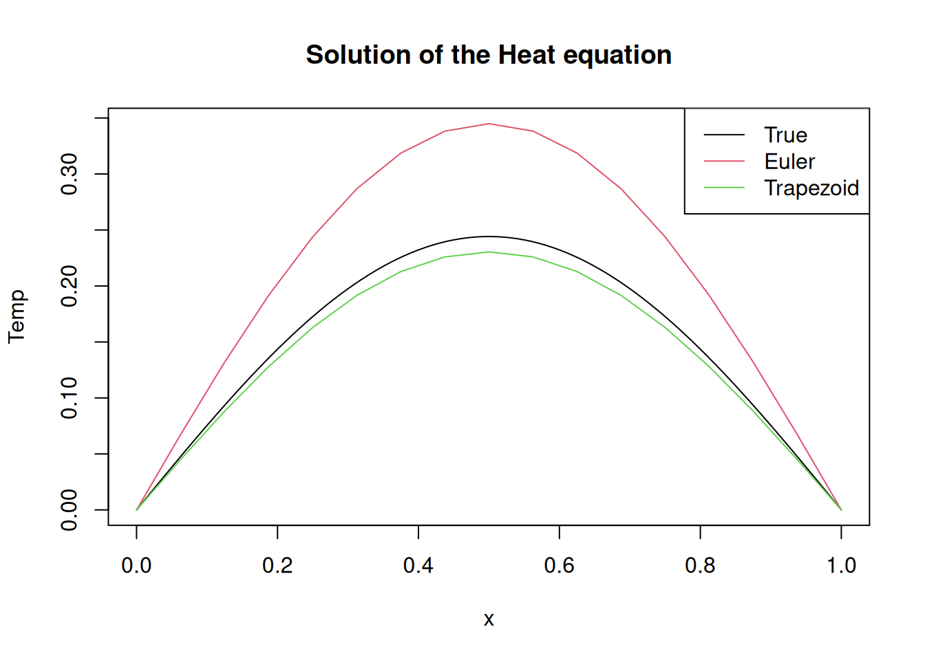
or for a given \(x\):
f2 <- function(t)
    exp(-pi^2*t)*sin(pi*x)
x <- res1$x[3]
Q <- curve(f2,0,1,main="Solution of the Heat equation",xlab="t",ylab="Temp")
lines(res1$t,res1$Theta[3,],col=2)
lines(res2$t,res2$Theta[3,],col=3)
legend("topright",c("True","Euler","Trapezoid"),col=1:3,lty=1) 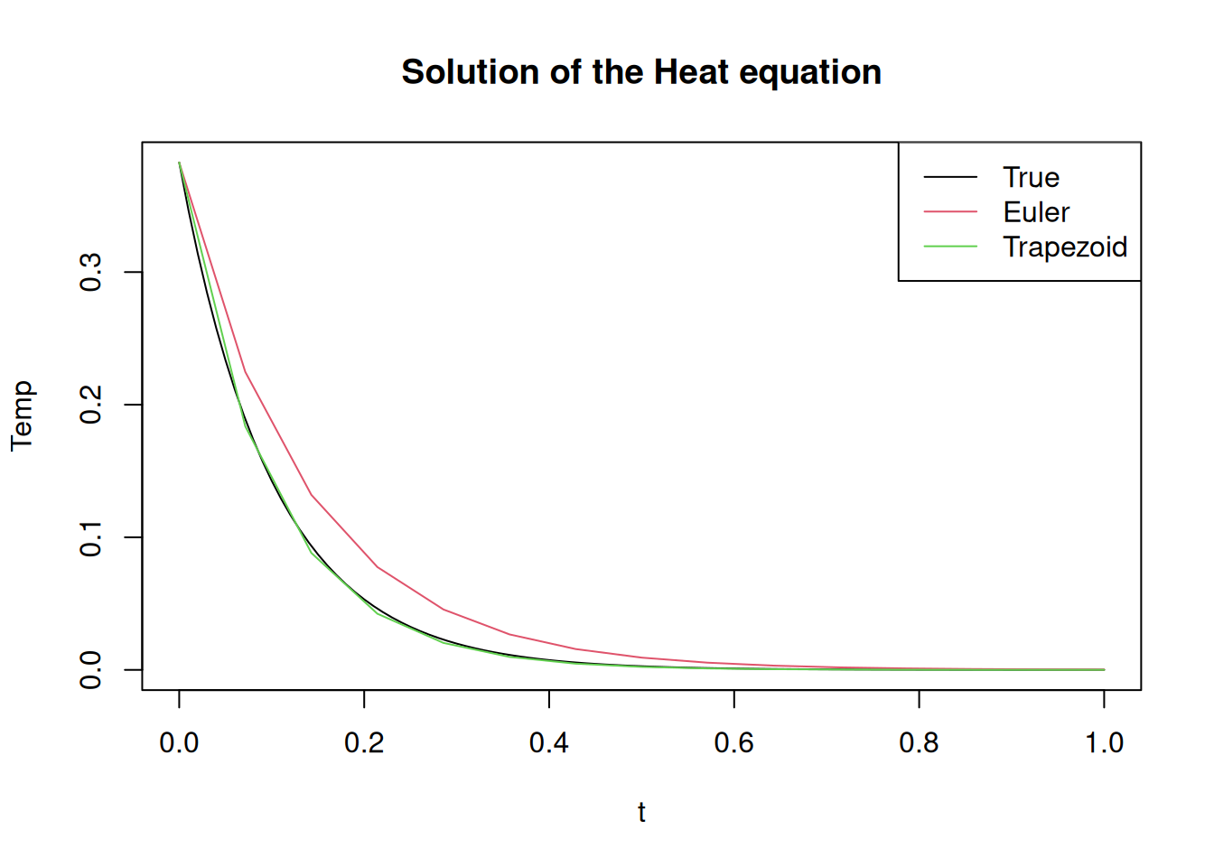
Exercise 8.5 Write a function that solve the Heat equation by using the Trapezoid rule. In a table, compare the error for different \(m\) and \(n\).
8.6 Black and Scholes and the Heat Equation
I only cover the theory briefly. For more details, see Hull (2011). We consider an European Call option. The exercise price is \(K\), the price of the underlying asset if \(S\), and the expiration date is \(T\). The value of such options at time \(t\) is \(V(S,t)\). We want to derive its relation with time and the price of the underlying stock. In the Black and Scholes’ formula, we assume that the stock price follows a geometric Brownian motion: \[ dS = S \mu dt + S\sigma dW \] and that we can construct a portfolio in which we go short one option and long \(dV/dS\) of the underlying asset. The value of this portfolio is \(\Pi=-V+S(dV/dS)\) and the return is \([-\Delta V+(dV/dS)\Delta S]/\Pi\). We can show that the portfolio is risk free, which implies that its return must be equal to the risk-free rate \(r\). By Ito’s Lemma, we have: \[ dV = \left( \mu S\frac{\partial V}{\partial S}+\frac{\partial V}{\partial t} + \frac{\sigma^2S^2}{2}\frac{\partial ^2V}{\partial S^2}\right)dt +\sigma S \frac{\partial V}{\partial S}dW \] By substituting \(dV\) and \(dS\) in \(\Delta \Pi\), we see that \(dW\) vanishes which implies the absence of risk. Using \(r\Pi dt=d\Pi\) with the above expression for \(\Pi\) and \(\Delta\Pi\), we get the partial differential equation of Black and Scholes. \[ \frac{\partial V}{\partial t} + \frac{\sigma^2S^2}{2}\frac{\partial ^2V}{\partial S^2} +r S \frac{\partial V}{\partial S} -rV = 0 \] with the condition: \(V(S,T)=(S-K)^+\), \(V(0,t)=0\) and \(V(S,t)\) converges to \(S\) as \(S\) goes to infinity. We can rewrite the partial differential equation as \(\theta_t=\theta_{xx}\) by the appropriate change of variables. Let \(x=log(S/K)\), \(\nu=V/K\), and \(\tau=(T-t)\sigma^2/2\). Then, we can write: \[ \frac{\partial \nu}{\partial \tau}=\frac{\partial^2\nu}{\partial x^2} + (k_1-1)\frac{\partial\nu}{\partial x}-k_1\nu \] with \(\nu(x,0)=(e^x-1)^+\), \(\nu(-\infty,\tau)=0\) and \(\nu(x,\tau)\approx S/K\) for large \(x\). Let \(\theta(x,\tau)=e^{-(\alpha x+\beta\tau)}\nu\), with \(\alpha=(1-k_1)/2\), and \(\beta=-(k_1+1)^2/4\), then the above equation can be written as: \[ \frac{\partial \theta}{\partial t} = \frac{\partial^2\theta}{\partial x^2} \]
Exercise 8.6 Consider an European Call option with exercise price \(K\), expiration date \(T\). The price of the underlying stock follows the process \(dS = S \mu dt + S\sigma dW\). Using the method to solve the Heat Equation, write a function that computes the value of the option \(V(t,S)\). Test it with different values of \(K\), \(T\), \(\sigma\), and \(\mu\). Compare your solution to the true formula. (suppose \(r=0.01\))
8.7 R packages for differential equations
Here is a list of existing packages:
- bvpSolve: Solvers for boundary value problems of ODEs
- ddesolve: Solver for Delay Differential Equations
- deSolve: General solvers for initial value problems of ordinary differential equations (ODE), partial differential equations (PDE), differential algebraic equations (DAE), and delay differential equations (DDE)
- deTestSet: Testset for differential equations
- odesolve: Solvers for Ordinary Differential Equations
- PBSddesolve: Solver for Delay Differential Equations
- rootSolve: Root finding, equilibrium and steady-state analysis of ODEs
- sde: Simulation and Inference for Stochastic Differential Equations
- Sim.DiffProc: Simulation of diffusion processes
- simecol: Simulation of ecological and other dynamic systems
I am not going to explain how these packages work. The manuals are detailed enough. Here is one example for boundary value problems using the bvpSolve (Soetaert, Cash, and Mazzia (2026)) and deSolve (Soetaert, Petzoldt, and Setzer (2026)) packages:
library(bvpSolve)
LifeCycle <- function(x,y,parms)
{
    rho<-0.04
    r <- 0.10
    gamma <- -2
    M <- 10
    R <- 40
    w <- (x<=R)*(x>=M)
    y1 <- r*y[2]+w-y[1]
    y2 <- (rho-r)*y[1]/gamma
    list(c(y2,y1))
}
init <- c(C=NA,A=0)
end  <- c(C=NA,A=0)
sol  <- bvpshoot(yini = init, x = seq(0, 55, by = 0.01),
                func = LifeCycle, yend = end,guess=.2)
And for initial value problem:
library(deSolve)
MGrowth3 <- function(x,y,parms)
    {
    res <- MGrowth2(x,y)
    list(res)}
y <- c(K=SteadyK*1.01,I=rep(-0.01,3))
sol <- rk4(y,MGrowth3,times=seq(0,73,length=400),parms=NULL)
plot(sol)