Chapter 5 Nonlinear Equations
5.1 One-dimensional problems
Consider the problem of computing the yield to maturity of a coupon-bond with semiannual coupon of $50, par value of $1,000, maturity of 10 years, and a price of $850. The formula that links the bond price and the yield is: \[ P = \frac{C}{y/2} + \left( PAR - \frac{C}{y/2}\right) (1+y/2)^{-2T}, \] where \(C\) is the coupon, \(y\) is the yield to maturity compounded semiannually, T is the maturity, and \(PAR\) is the par value. In our problem, we want to solve: \[ f(y) = 850 - \frac{50}{y/2} - \left( 1000 - \frac{50}{y/2}\right) (1+y/2)^{-20} = 0 \] The following graph shows the shape of \(f(y)\):
f <- function(y)
    850-50/(y/2)-(1000-50/(y/2))*(1+y/2)^(-20)
y <- seq(0.01,.3,len=100)
P <- f(y)
plot(y,P,main="Coupon-Bond:  Price = f(Yield)",
xlab="Yield",ylab="Price",type="l")
abline(h=0)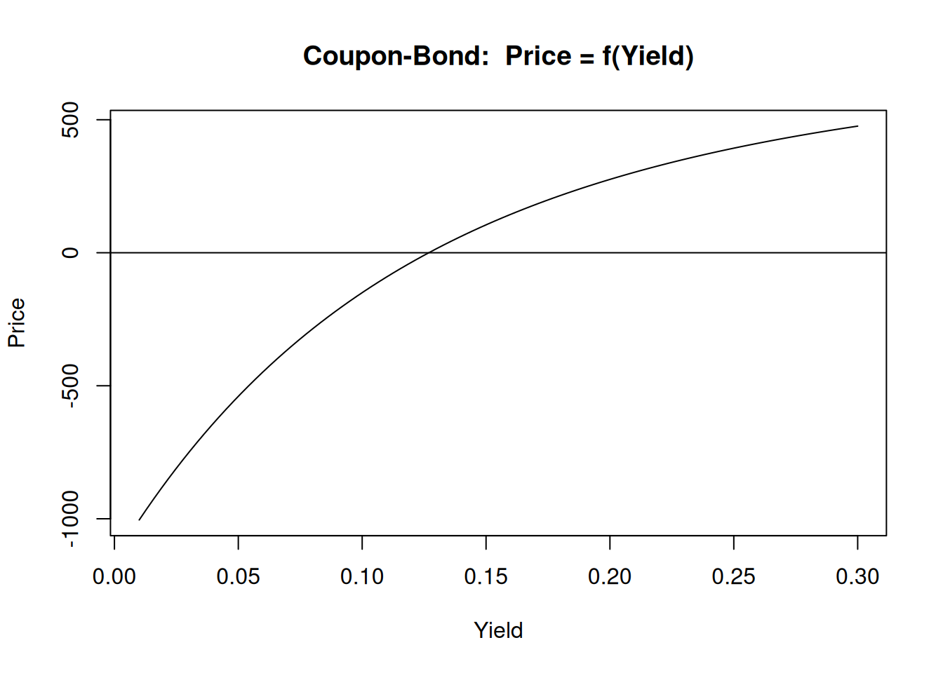
One possibility is to solve the problem using a grid-search. In the above example, we know that the solution must be between 0 and 1, which makes it easy to construct the grid. The following function is an example of how to do it. The stopping rule is: stop if a) \(f(x_i)<0\), \(f(x_j)>0\) ,and either b) \(\max(x_i,x_j)-min(x_i,x_j) < \epsilon (1 + |x_i| + |x_j|)\), or c) \(|f((x_i+x_j)/2)| < \delta\).
YieldGrid <- function(from, to, n, eps=1e-6, delta=1e-6, maxit=100, P=850, PAR=1000,
                      C=50, N=2, T=10)
{
    f <- function(y)
        P-C/(y/N)-(PAR-C/(y/N))*(1+y/N)^(-N*T)
    y <- seq(from, to, len=n)
    fVal <- f(y)
    neg <- fVal<0
    if (all(neg) | all(!neg))
        stop("There is no solution between from and to")
    t <- 1
    while (TRUE)
  {
        if (neg[1])
        {
            to <- y[which(!neg)][1]
            from <- y[which(!neg)-1][1]
        }   else {
            to <- y[which(neg)][1]
            from <- y[which(neg)-1][1]
        }
    check <- (to-from)<eps*(1+abs(from)+abs(to)) | abs(f((from+to)/2))<delta
        if(t>=maxit)
        {
            mess <- "No convergence: maxit reached"
            break
        }
        if (check)
        {
            mess <- paste("Converged after ",t," iterations",sep="")
            break
        }
        y <- seq(from, to, len=n)
        fVal <- f(y)
        neg <- fVal<0
        t <- t+1
    }
    ans <- list(sol=(from+to)/2,fct=f((from+to)/2),message=mess,iter=t,
                name="Grid Search for Yield to Maturity",prec=to-from)
    class(ans) <- "Zeros"
    return(ans)
}

print.Zeros <- function(obj)
{
    cat("\nMethod: ",obj$name,"\n")
    cat("Message: ", obj$mess,"\n\n")
    if(length(obj$sol)==1)
    {
        cat("The solution is: ",obj$sol,", and f(x) is ",obj$fct,"\n")
    } else {
        cat("The solution is: \n")
        if(is.null(names(obj$sol)))
            names(obj$sol) <- paste("x",1:length(obj$sol),sep="")
        for(i in 1:length(obj$sol))
            cat(names(obj$sol)[i]," = ",obj$sol[i],"\n")
        cat("\nf(x) is ",obj$fct,"\n")
    }
    cat("Precision: ",obj$prec,"\n")
}
The function is for general case and it produces an object of class “Zeros”. All algorithms of this chapter will produce the same type of object, The solution is:
##
## Method:  Grid Search for Yield to Maturity
## Message:  Converged after 6 iterations
##
## The solution is:  0.1268917 , and f(x) is  1.666213e-07
## Precision:  7.152515e-11
The method converges after 6 iterations. It may look efficient at first but since there are 50 function evaluations per iteration, the solution is reached after 300 function evaluations. We can do much better than that.
5.1.1 The Bisection Method {#chap5-1-1
There is no closed-form solution to the above problem, bu we can easily find the solution using a bracketing method called the Bisection. All we need is two points \(a<b\) that are such that the signs of \(f(a)\) and \(f(b)\) are different. We then consider a third point \(c=(a+b)/2\), and replace \(a\) by \(c\) if the sign of \(f(a)\) and \(f(c)\) are the same, and inversely if the signs of \(f(b)\) and \(f(c)\) are the same. The Stopping rule is: stop if either \(b-a < \epsilon (1 + |a| + |b|)\), or \(|f((a+b)/2)| < \delta\). The following function computes the zero of a function between \(a\) and \(b\) using that method:
Bisection <- function(f,a,b,eps=1e-7,delta=1e-7,maxit=100)
{
    fa <- f(a); fb <- f(b); t <- 1
    if (a>=b)
        stop("a must be strictly smaller than b")
    if(fa*fb>=0)
        stop("f(a) and f(b) have different signs")
    res <- vector()
    while(TRUE)
    {
        fc <- f(c <- (a+b)/2)
        if (fa*fc>0)
        {
            a <- c
            fa <- fc
        } else {
            b <- c
            fb <- fc
        }
        res <- rbind(res,c(c,fc))
        if(t>=maxit)
        {
            mess <- "No convergence: maxit reached"
            break
        }
        check <- (b-a)<eps*(1+abs(a)+abs(b)) | abs(fc)<delta
        if (check)
        {
            mess <- paste("Converged after ",t," iterations",sep="")
            break
        }
        t <- t+1
    }
    ans <- list(sol=c,fct=fc,message=mess,iter=t,name="Bisection",prec=(b-a),x=res)
    class(ans) <- "Zeros"
    return(ans)
}
We can then try it using the same problem:
f <- function(y,P=850, PAR=1000, C=50, N=2, T=10)
    P-C/(y/N)-(PAR-C/(y/N))*(1+y/N)^(-N*T)
Bisection(f,.01,1)
##
## Method: Bisection
## Message: Converged after 23 iterations
##
## The solution is: 0.1268917 , and f(x) is -0.0004022902
## Precision: 1.180172e-07It is much better than the grid search if we consider that the algorithm evaluated the function only 23 times. The following graph shows the convergence of the method.
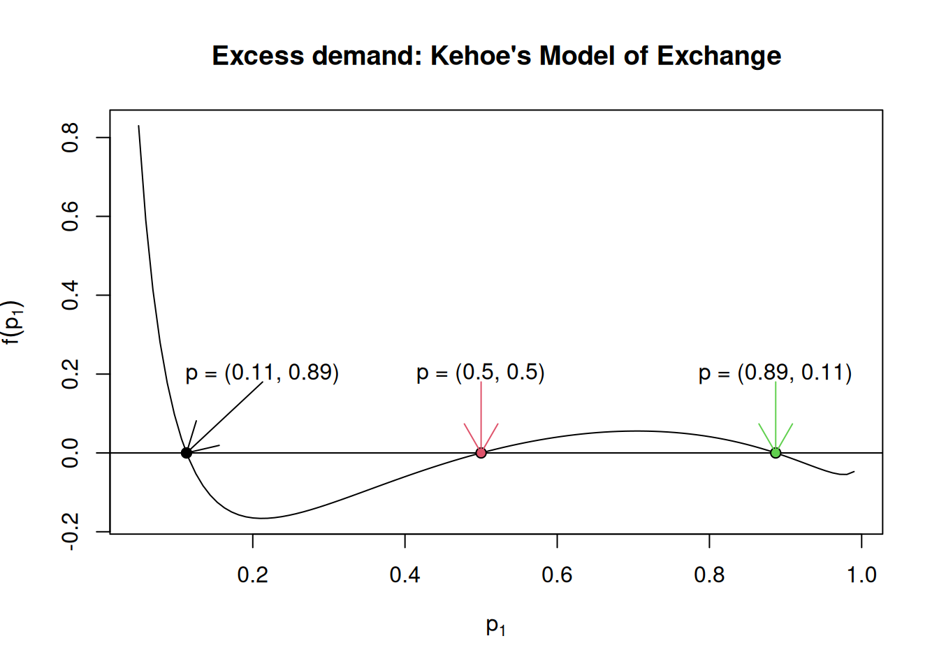
The solution of course depends on the choice of \(a\) and \(b\). Is there are multiple solutions, it will find one solution in \([a,b]\). To see that, consider an exchange economy with 2 goods and 2 agents. The utility of agent \(i\) is (page 154 of Judd (1998)): \[ u_i(x_1,x_2) = \frac{a_1^ix_1^{\gamma_i+1}}{\gamma_i+1} + \frac{a_2^ix_2^{\gamma_i+1}}{\gamma_i+1}~~~,i=1,2, \] where \(a_j^i\geq 0\), and \(\gamma_i<0\). Let \(\eta_i = -1/\gamma_i\), \(e^i=\{e_1^i,e_2^i\}\) be the endowment of agent \(i\), and \(Y^i=p_1e_1^i+p_2e_2^i\) be the income of agent \(i\). The equilibrium condition is \(d_j^1(p)+d_j^2(p) = e_j^1+e_j^2\) for goods \(j=1,2\). By Walras’s law, we only need to solve for one of the two goods. If we normalize the prices such that \(p_1+p_2=1\), the equilibrium condition is: \[ f(p_1) = d_1^1(p_1,1-p_1)+d_1^2(p_1,1-p_1) - e_1^1 - e_1^2 = 0 \] with \[ d_1^1(p_1,1-p_1) = \frac{(a_1^1)^{\eta_1}}{(a_1^1)^{\eta_1}p_1^{1-\eta_1} + (a_2^1)^{\eta_1}(1-p_1)^{1-\eta_1}} Y^1p_1^{-\eta_1} \] \[ d_1^2(p_1,1-p_1) = \frac{(a_1^2)^{\eta_2}}{(a_1^2)^{\eta_2}p_1^{1-\eta_2} + (a_2^2)^{\eta_2}(1-p_1)^{1-\eta_2}} Y^2p_1^{-\eta_2} \]
To solve the problem, I am constructing a new object of type utility, and we define two agents with the parameter values determined on page 154 of Judd (1998).
CES <- function(par)
{
    names(par) <- NULL; good=TRUE
    if(length(par)!=5 | par[3]>=0 | any(par[1:2]<0) | any(par[4:5]<0))
        good <- FALSE
    par <- c(a=par[1:2],gamma=par[3],eta=-1/par[3],e=par[4:5])
    f <- expression(a1*x1^(gamma+1)/(gamma+1) + a2*x2^(gamma+1)/(gamma+1))
    X1 <- expression(
            (a1^eta/(a1^eta*p1^(1-eta) + a2^eta*p2^(1-eta)))* (p1*e1+p2*e2) * p1^(-eta))
    X2 <- expression(
            (a2^eta/(a1^eta*p1^(1-eta) + a2^eta*p2^(1-eta)))* (p1*e1+p2*e2) * p2^(-eta))
    Y <- expression(e1*p1+e2*p2)
    Indif <- expression( ( ((gamma+1)*U-a1*x1^(gamma+1))/a2 )^(1/(gamma+1)) )
    fct <- paste("U = (", par[1], "*X1^",par[3]+1," + ", par[2],"*X2^",
                 par[3]+1,"/(",par[3]+1,sep="")
    ans <- list(Uexp = f, Sol=list(X1=X1,X2=X2),par=par,name="CES",
            fct=fct,Indif=Indif,good=good,Y=Y)
    class(ans) <- "Utility"
    return(ans)
}
cons1 <- consumer("John",c(1024,1,-5,12,1),utility="CES")
cons2 <- consumer("Bill",c(1,1024,-5,1,12),utility="CES")We can then easily compute the function that defines the equilibrium condition:
Kehoe <- function(p1)
{
    d1 <- sapply(1:length(p1), function(i) solve(cons1,c(p1[i],1-p1[i]),F)$x1)
    d2 <- sapply(1:length(p1), function(i) solve(cons2,c(p1[i],1-p1[i]),F)$x1)
    d1+d2-cons1$par[4]-cons2$par[4]
}
The following graph shows the shape of the excess demand function. There are three possible equilibria.
If we try to solve it using the above Bisection method using different \(a\) and \(b\), we obtain:
##
## Method:  Bisection
## Message:  Converged after 22 iterations
##
## The solution is:  0.1129238 , and f(x) is  2.06554e-07
## Precision: 9.298325e-08##
## Method: Bisection
## Message: Converged after 19 iterations
##
## The solution is: 0.5000002 , and f(x) is 9.765621e-08
## Precision: 5.722046e-07##
## Method: Bisection
## Message: Converged after 19 iterations
##
## The solution is: 0.8870762 , and f(x) is -2.175291e-08
## Precision: 3.814697e-07Easy when we know the solutions. If the interval contains more than one solution, the result is uncertain:
##
## Method:  Bisection
## Message:  Converged after 23 iterations
##
## The solution is:  0.1129239 , and f(x) is  -1.799073e-07
## Precision: 1.060963e-07##
## Method: Bisection
## Message: Converged after 1 iterations
##
## The solution is: 0.5 , and f(x) is 3.552714e-15
## Precision: 0.49##
## Method: Bisection
## Message: Converged after 21 iterations
##
## The solution is: 0.887076 , and f(x) is 9.026282e-08
## Precision: 4.243851e-075.1.2 Newton’s Method
For the Newton’s method, we first get the linear approximation of \(f(x)\) around \(x_0\), and find the zero of the linear function. We have \(f(x)\approx f(x_0) + f'(x_0)(x-x_0)=0\) , which implies that \(x= x_0 - f(x_0)/f'(f_0)\). The algorithm is therefore: \[ x_{k+1}=x_k - \frac{f(x_k)}{f'(x_k)} \] The stopping rule is similar to the one we used in the last chapter except that we want to check if \(f(x_{k+1})=0\) is satisfied instead of \(f'(x_{k+1})=0\). So we stop if \(|x_k-x_{k+1}|<\epsilon(1+|x_{k+1}|)\) and conclude that we have a solution if \(|f(x_{k+1}|<\delta\). I wrote a function to compute the solution using the Newton’s Method. I don’t show it to you because it is the next exercise. The function requires as arguments, \(f(x)\) and \(df(x)\). We can test it using the the above examples.
##
## Method:  Newton
## Message:  Converged after 6 iterations
##
## The solution is:  0.1268917 , and f(x) is  0
## Precision: 6.642408e-10##
## Method: Newton
## Message: No convergence: maxit reached (Bad convergence, f(x) not zero)
##
## The solution is: 0.5129672 , and f(x) is 0.006465041
## Precision: 0.01818518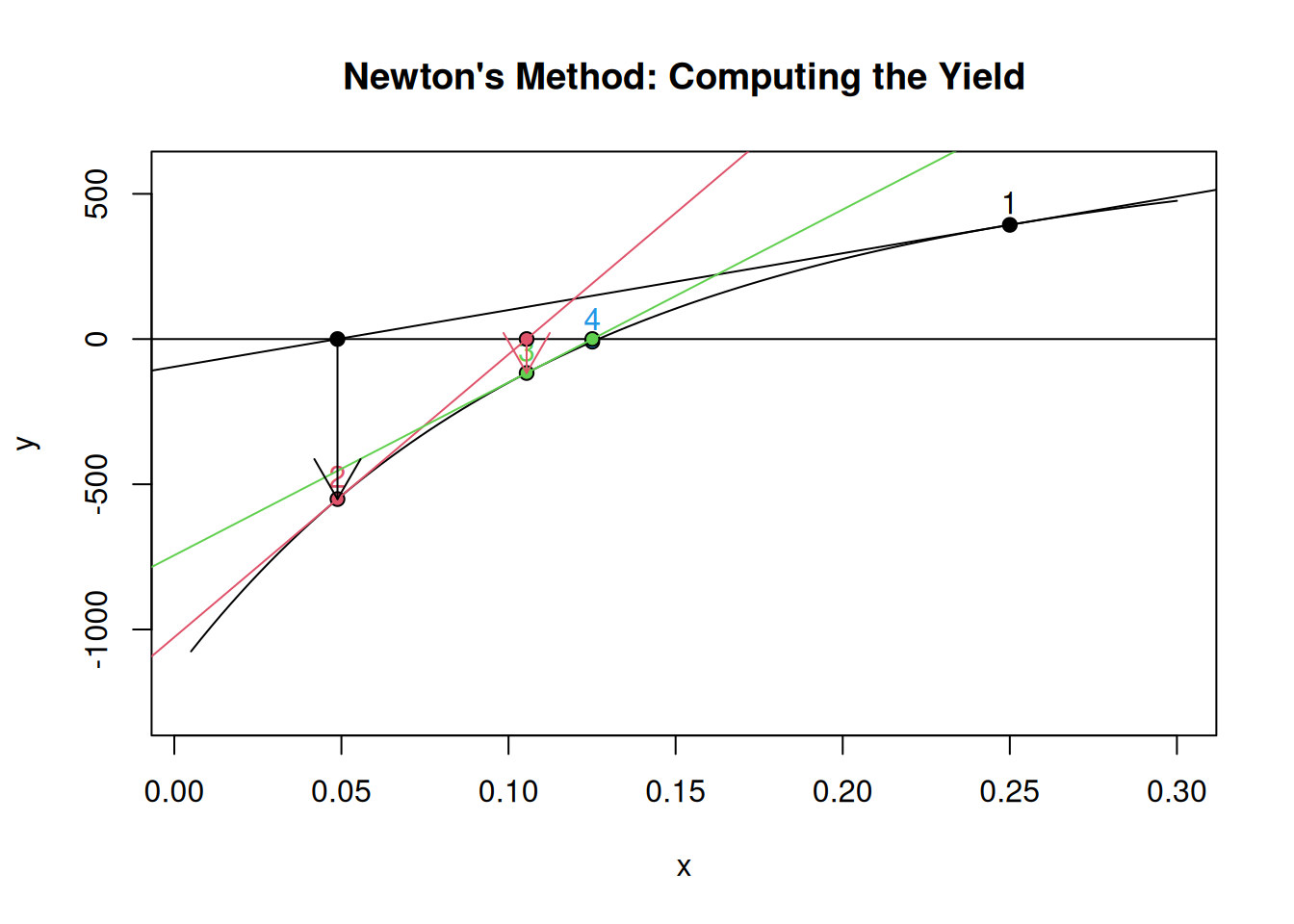
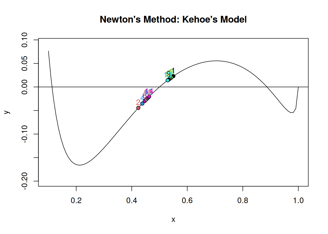
The method works fine for the Yield problem, but not for the Kehoe’s model. We can see on the graph that it gets stuck in a cycle around the solution. This result depends on the properties of the function around the solution. If we try another starting value, we see that the first equilibrium can easily be found. But for many starting values, the Newton’s method diverges (try it).
##
## Method:  Newton
## Message:  Converged after 8 iterations
##
## The solution is:  0.1129238 , and f(x) is  3.594499e-08
## Precision:  5.734584e-08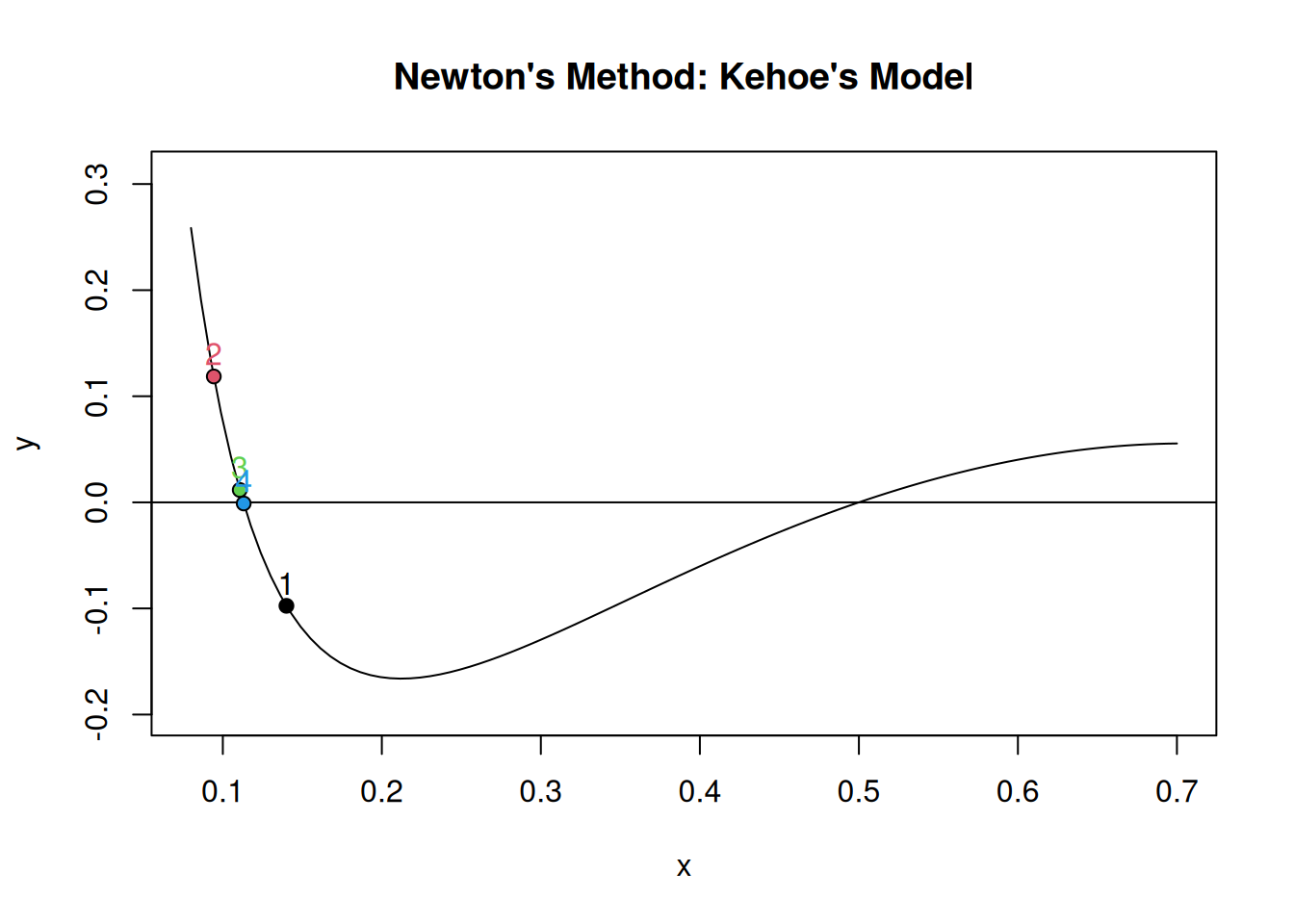
Exercise 5.1 Write a function that solve \(f(x)=0\) using the Newton’s Method. Test it on the previous examples.
Exercise 5.2 Write a function that solve \(f(x)=0\) using the Newton’s Method with acceleration or stabilization parameter \(\omega\). Test it on the previous examples.
5.2 Multivariate Nonlinear Equations
Here, we consider methods to solve \(f(x)=0\), where \(f\) is a function from \( \mathbb{R} ^n\) to \( \mathbb{R} ^n\). We consider the following Duopoly problem: There are two goods, \(X\) and \(Z\), and the utility of consumers is \[ U = u(Y,Z) + M = (1+Y^\alpha + Z^\eta)^{\eta/\alpha} + M \] The profit functions of firm \(Y\) and \(Z\) are: \[ \Pi^Y(Y,Z) = u_y(Y,Z) Y - C_YY, \] and \[ \Pi^Z(Y,Z) = u_z(Y,Z) Z - C_zZ. \] The first order condition is: \[ \frac{\partial \Pi^Y(Y,Z)}{\partial Y} = 0 \] and \[ \frac{\partial \Pi^Z(Y,Z)}{\partial Z} = 0 \] My function produces a vector \(f(x)\) or the Jacobian \(J(x)\).
Pi <- function(x,d=0)
{
    Y <- exp(x[1])
    Z <- exp(x[2])
    alpha <- 0.999; eta <- .2
    Cy <- .07; Cz <- .08
    U <- expression((1+Y^alpha+Z^alpha)^(eta/alpha))
    dUy <- D(U,"Y")
    Piy <- paste(dUy[2],dUy[1],dUy[3],"*Y-Cy*Y",sep="")
    Piy <- parse(text=Piy)
    dUz <- D(U,"Z")
    Piz <- paste(dUz[2],dUz[1],dUz[3],"*Z-Cz*Z",sep="")
    Piz <- parse(text=Piz)
    dPiy <- D(Piy,"Y")
    dPiz <- D(Piz,"Z")
    if (d==0)
    {
        c(eval(dPiy),eval(dPiz))
    } else {
        J <- c(eval(D(dPiy,"Y")),eval(D(dPiz,"Y")),
               eval(D(dPiy,"Z")),eval(D(dPiz,"Z")))
        matrix(J,2,2)
    }
}
5.2.1 Newton’s Method
The multivariate version of the Newton’s method is: \[ x_{k+1} = x_k - J(x_k)^{-1}f(x_k) \]
NewtonMNL <- function(f,x0,eps=1e-7,delta=1e-7,maxit=100)
{
    t <- 1
    f0 <- f(x0)
    df0 <- f(x0,1)
    while(TRUE)
    {
        x <- x0-solve(df0,f0)
        f0 <- f(x)
        df0 <- f(x,1)
        if(t>=maxit)
        {
            mess <- "No convergence: maxit reached"
            break
        }
        check <- sqrt(crossprod(x-x0)) < eps*(1+sqrt(crossprod(x0)))
        if (check)
        {
            mess <- paste("Converged after ",t," iterations",sep="")
            break
        }
        t <- t+1
        x0 <- x
    }
    if (sqrt(crossprod(f0))>delta)
        mess <- paste(mess," (Bad convergence, f(x) not zero)",sep="")
    ans <- list(sol=x,fct=f0,message=mess,iter=t,
                name="Multivariate Newton for Nonlinear System",
                prec=sqrt(crossprod(x-x0))/(1+sqrt(crossprod(x0))))
    class(ans) <- "Zeros"
    return(ans)
}##
## Method: Multivariate Newton for Nonlinear System
## Message: Converged after 22 iterations
##
## The solution is:
## x1 = -0.1374651
## x2 = -0.5759185
##
## f(x) is 4.646666e-10 2.077254e-09
## Precision: 5.820559e-085.2.2 Gauss Methods
As for the linear case, you can solve the problem using methods such as Gauss-Jacobi or Gauss-Seidel. They replace the n-dimensional problem by \(n\) one-dimensional problems. There are two possible approaches. In the first, the one-dimensional problems are solve completely, and in the second, they are solved using a linear approximation. For the Gauss-Jacobi, we obtain \(x_i^{k+1}\) either by solving
\[
f(x_{-i}^k,x_i^{k+1})=0
\]
or using the the Taylor approximation:
\[
x_i^{k+1} = x_i^k - \frac{f^i(x^k)}{f^i_{x_i}(x_k)}
\]
For the Gauss-Seidel, we update the \(x_i^k\) as soon as there are available. I give you the result using the function I wrote. You have to write your own function as an exercise.
##
## Method:  Gauss-Jacobi for Nonlinear System
## Message:  Converged after 17 iterations
##
## The solution is:
## x1  =  -0.1374662
## x2  =  -0.5759235
##
## f(x) is  7.309127e-08 1.641704e-07
## Precision:  5.029531e-09
##
## Method: Gauss-Seidel for Nonlinear System
## Message: Converged after 9 iterations
##
## The solution is:
## x1 = -0.1374662
## x2 = -0.5759236
##
## f(x) is 7.311276e-08 1.642665e-07
## Precision: 2.692622e-09##
## Method: Linear Gauss-Jacobi for Nonlinear System
## Message: Converged after 32 iterations
##
## The solution is:
## x1 = -0.1374652
## x2 = -0.5759184
##
## f(x) is 1.217085e-10 -4.077542e-10
## Precision: 9.638562e-09##
## Method: Linear Gauss-Seidel for Nonlinear System
## Message: Converged after 28 iterations
##
## The solution is:
## x1 = -0.1374651
## x2 = -0.5759184
##
## f(x) is 1.028884e-10 -2.664104e-10
## Precision: 8.026069e-09Exercise 5.3 Write a function to solve the system of n equations \(f(x)=0\) using the Gauss-Jacobi and Gauss-Seidel methods. For solving the one-dimensional problems, use the R function uniroot
Exercise 5.4 Write a function to solve the system of n equations \(f(x)=0\) using the linear approximation version of the Gauss-Jacobi and Gauss-Seidel methods.
5.2.3 Broyden’s Method
The Broyden’s method is similar to the Newton’s method with the exception that it approximate the Jacobian and update it at each iteration as the BFGS method does for the Hessian matrix. Let \(A_k\) be the approximation of \(J(x_k)\), starting with \(A_0=I\), the update is: \[ A_{k+1} = A_k + \frac{(y_k-A_ks_k)s_k'}{s_k's_k} \] where \(y_k=f(x_{k+1})-f(x_k)\). The idea is to have a matrix \(A_{k+1}\) that satisfies \(A_{k+1}s_k=f(x_k+s_k)-f(x_k)\), a properties that is satisfied by the Jacobian. In fact, for any direction \(q\), \(J(x)q\) approximates \(f(x+q)-f(x)\). In the one dimensional case, we have \(f'(x)h\approx f(x+h)-f(x)\). You can verified that the above updating scheme satisfies \(A_{k+1}s_k=y_k\).
##
## Method:  Broyden's Method
## Message:  Converged after 36 iterations
##
## The solution is:
## x1  =  -0.1374651
## x2  =  -0.5759184
##
## f(x) is  -1.434131e-11 1.172108e-11
## Precision:  6.79486e-08
As it is expected, the approximated Jacobian makes it a little slower than the Newton’s Method. The advantage is for large systems because it avoids the computation of the Jacobian at each iteration for which the number of operations is of order \(n^2\).
Exercise 5.5 Write a function that solves \(f(x)=0\), for \(f(x): \mathbb{R} ^n\rightarrow \mathbb{R} ^n\), using the Broyden’s Method. Test your method on the above duopoly example.
5.2.4 The nleqslv package
The nleqslv package (Hasselman and Carnell (2026)) provides functions for solving systems of nonlinear equations. The main function is nleqslv, which uses either the Newton or the Broyden’s method. The function uses a method similar to the one we saw in the last chapter for improving the convergence speed. The updating scheme is \(x_{k+1}=x_k+\lambda s_k\). The lambda is selected using a kind of line search. The criterion is base on the impact of the step on \(f(x)'f(x)\). The options are:
- The first three are respectively \(x_0\), \(f\) and \(J\), where \(f\) and \(J\) are functions.
- method = either “Broyden” of “Newton”
- global = different method for selecting the \(\lambda\). You can choose “none” if you want \(\lambda=1\)
- xscalm = method for re-scaling the \(x\)’s. You always make sure the \(x_i\)’s have comparable scales.
- control = list(): Many parameter to adjust if you want. For example, xtol and ftol are what we call \(\epsilon\) and \(\delta\) in the above algorithms, maxit the number of iterations, trace=1 will print the details of each iterations, and a bunch of other tuning parameters.
To see how it works, we apply it to the duopoly problem.
## $x
## [1] -0.1374651 -0.5759186
##
## $fvec
## [1] -1.782566e-09  3.254971e-09
##
## $termcd
## [1] 1
##
## $message
## [1] "Function criterion near zero"
##
## $scalex
## [1] 1 1
##
## $nfcnt
## [1] 15
##
## $njcnt
## [1] 1
##
## $iter
## [1] 12
See the help file to understand all codes. In particular we see that there is only one Jacobian evaluation (because it is the Broyden’s Method) and 15 function evaluations.
5.2.5 Application
Consider the endowment economy in which there are \(m\) goods, and \(n\) agents with utilities: \[ u^i(x) = \sum_{j=1}^m \frac{a_{ij}x_j^{v_{ij}+1}}{1+v_{ij}},~~i=1,...,n, \] endowed with \(e_{ij}\) units of good \(j\), where \(m=n=10\), and the coefficients are obtained randomly as follows (for \(a\), \(e\) and \(v\), the \(i^{th}\) row is for the \(i^{th}\) agent and the \(j^{th}\) column the \(j^{th}\) good):
set.seed(445)
n <- 10
m <- 10
a <- matrix(runif(n*m,1,10),n,m)
v <- matrix(runif(n*m,-3,-0.5),n,m)
e <- matrix(runif(n*m,1,5),n,m)
By using Walras law and the normalization \(\sum_{i=1}^m p_i=1\), the problem is to solve the following equations: \[ \begin{split} E_1(p)=&0\\ E_2(p)=&0\\ \vdots\\ E_{m-1}(p)=&0\\ \sum_{i=1}^m p_i =& 1, \end{split} \] where \(E_i(p)\) is the excess demand of good \(i\).
Exercise 5.6 Solve the equilibrium problem of the above endowment economy. Use the algorithm that you want but \(E_i(p)\) must be obtained numerically using the optimizer of your choice.