Chapter 7 Monte Carlo Simulation
7.1 Introduction
We want to look at methods to compute integrals or to solve optimization problems based on simulations. Here is a simple example. Suppose you want to compute the value of \(\pi\). We all know that it is the area of a unit circle. But it is also the probability of being in a unit circle inside a \(2\times 2\) square if we randomly draw numbers uniformly over the square times the area of the square, which is 4. The following figure shows the idea.
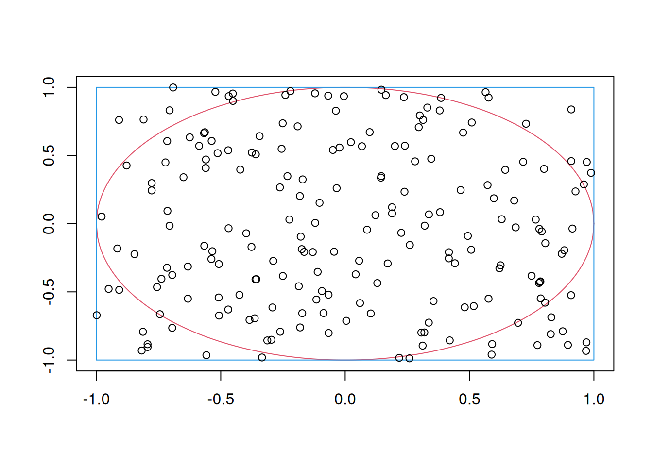
By counting the proportion of points in the circle, we estimate \(\pi\):
## [1] 3.141298It is accurate up to 3 decimals. As you see, we need a lot of points to get that level of accuracy. In some problems, however, Monte Carlo simulations are the only feasible way to get an estimate of the solution we are looking for.
In order to perform Monte Carlo simulations, we need a random number generator. Such generators do not exist in practice. We use pseudo-random generators, which are deterministic formulas that generate numbers that approximate the properties of random numbers. That’s the reason some purists will call these methods pseudo Monte Carlo to point out that we are not using real random numbers. A uniform pseudo random number can be generated as: \[ X_{k+1} = aX_{k}+b~ (mod~m), \] where \(N ~(mod~m)\) is the remainder of \(N/m\), and \(X_0\) is called the seed and must be an odd number. Therefore, for any given seed, we have the same sequence of pseudo random number. For example, consider the following homemade pseudo random generator:
myUnif <- function(n,a,c,m,seed)
{
    seed <- (seed%/%2)*2+1
    x <- seed
    for (i in 2:(n+1))
        x[i] <- (x[i-1]*a+c) %% m
    return(x[-1]/m)
}
We can see on the following figure that the function produces numbers between 0 and 99 (because \(0\leq N~(mod~m) \leq (m-1)\)) that look random.
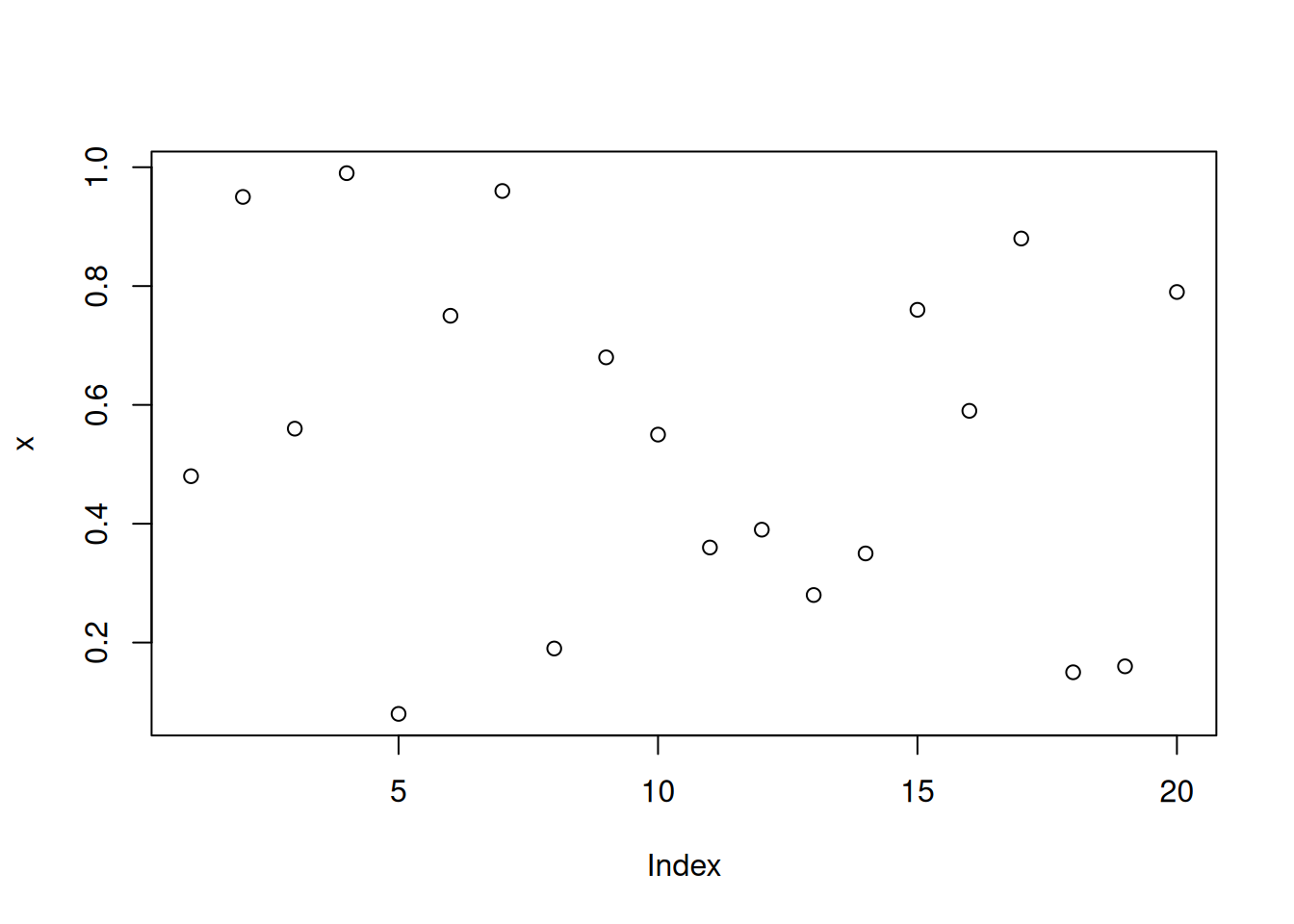
However, the sequence has a period of 20:
##      [,1] [,2]
## [1,] 0.48 0.48
## [2,] 0.95 0.95
## [3,] 0.56 0.56
## [4,] 0.99 0.99
## [5,] 0.08 0.08
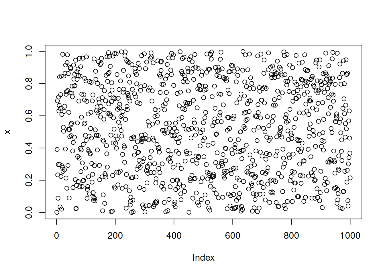
To get a longer sequence we have to change the seed every 20 numbers. Here is a much realistic choice of the parameters (the period is 5.3687091^{8}):
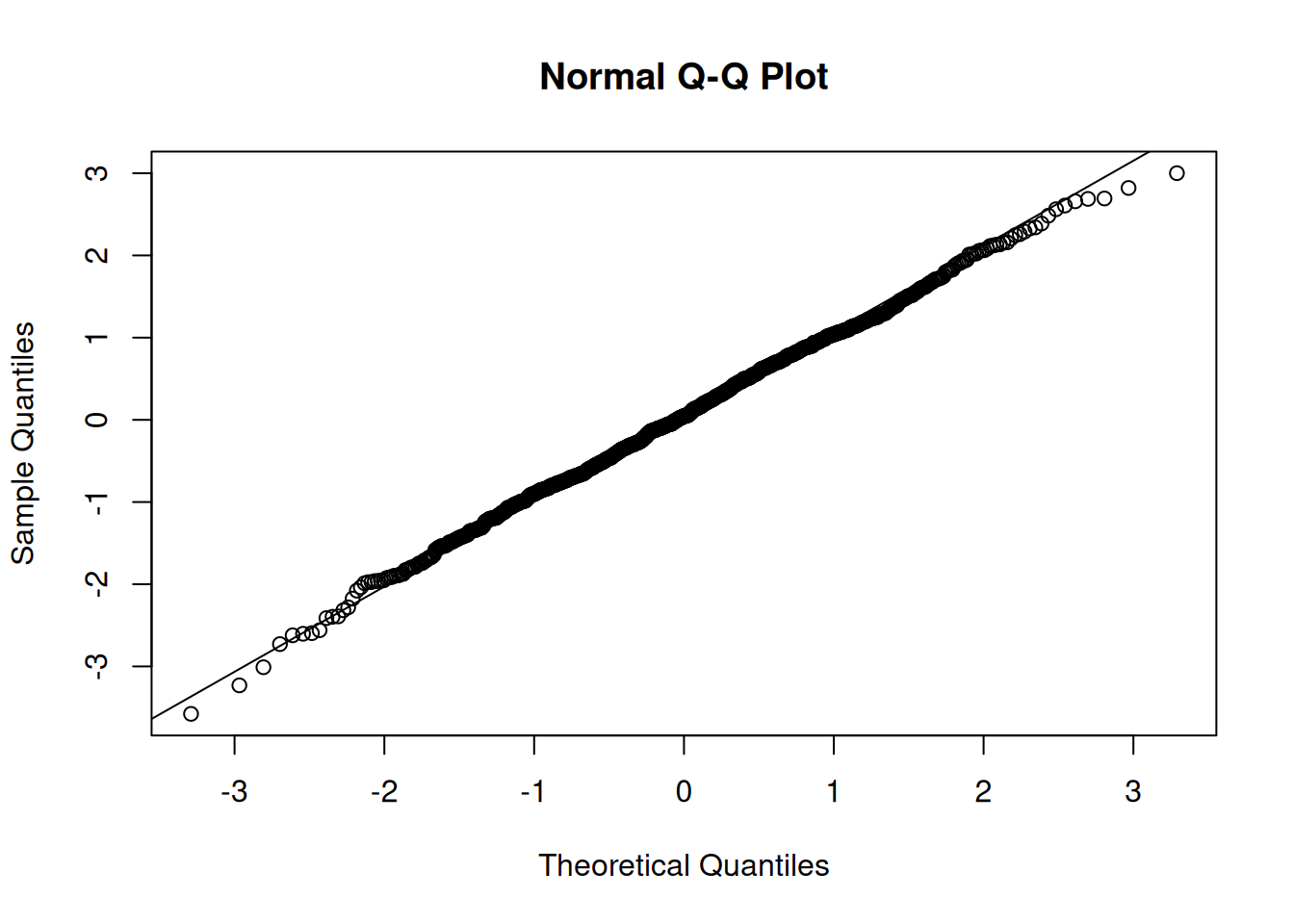
We call them pseudo random numbers because they are perfectly predictable once we know the seed. Other pseudo random numbers can be generated using the following. Let \(F()\) be a distribution function. If \(x\sim U(0,1)\), then \(y = F^{-1}(x)\) has a distribution function \(F(y)\). We can then construction a \(N(0,1)\) pseudo random number as follows:
7.2 Econometrics
We first look at some examples of Monte Carlo simulations in econometrics. In fact, many think that those numerical experiments are reserved to econometrics. We will see that it is not the case in the next sections.
One application is to analyze the properties of estimators. For example, the OLS estimator of the regression \(Y=X\beta+u\), can be written as: \[ \hat{\beta} = \beta + (X'X)^{-1}X'u \] We want to show that \(\hat{\beta}\) is biased whenever \(E(u|x)\neq 0\). In other words we want to measure \(E(\hat{\beta})\) and see if it is equal to \(\beta\). But \(E(\hat{\beta})\) is: \[ E(\hat{\beta}) - \beta = \int \cdots \int (X'X)^{-1}X'u f(x_1,x_2,...,x_k,u) dx_1\cdots dx_kdu \] We could assume a distribution \(f(x_1,x_2,...,x_k,u)\) and compute the integral, but it would be hard for large systems. What we do instead, we generate samples, estimate \(\hat{\beta}\) for each sample, and compute the sample mean of the \(\hat{\beta}\)’s. By the law of large numbers, this method should give us a consistent estimate of \(E(\hat{\beta})\). For example, suppose that \(u\sim N(0,1)\), \(X_1\sim U(0,1)\), \(X_2=.4u+2Z+U(0,1)\), \(Z\sim U(0,1)\), and \(Y=1+2X_1+3X_2+u\). We don’t know the joint distribution of \(X_1\), \(X_2\), and \(u\). It is therefore hard to compute the integral. The Monte Carlo approach, however, is not too hard. We can compare the bias of OLS and GMM with 500 iterations and a sample size of 50. Notice that we would get a better estimate by increasing the number of iterations.
library(gmm)
library(parallel)
set.seed(123)
n <- 50
N <- 500
u <- matrix(rnorm(n*N),n,N)
x1 <- matrix(runif(n*N),n,N)
Z <- matrix(runif(n*N),n,N)
x2 <- .4*u + 2*Z + matrix(runif(n*N),n,N)
y <- 1+2*x1+3*x2+u
beta <- mclapply(1:N,function(i) lm(y[,i]~x1[,i]+x2[,i])$coef, mc.cores = 16)
beta_GMM <- mclapply(1:N, function(i) {
      dat <- data.frame(y=y[,i], x1=x1[,i], x2=x2[,i], Z = Z[,i])
      fit <- gmm(y~x1+x2,~x1+Z, data=dat)
      coef(fit)}, mc.cores = 16)
beta <- do.call(cbind, beta)
beta_GMM <- do.call(cbind, beta_GMM)
bias <- rowMeans(beta)-c(1,2,3)
names(bias) <- c("b0","b1","b2")
bias <- rbind(bias,rowMeans(beta_GMM)-c(1,2,3))
rownames(bias) <- c("OLS","GMM")| b0 | b1 | b2 | |
|---|---|---|---|
| OLS | -1.0689 | 0.0293 | 0.6965 |
| GMM | -0.0099 | 0.0226 | -0.0043 |
Computing biases and variances of estimators for small samples can only be done using Monte Carlo methods, because all we know about estimators in practice is how they behave when the sample size goes to infinity; thanks to the several central limit theorems and laws of large numbers. For example, GMM estimators are asymptotically unbiased, but in small samples, the bias increases with the number of moment conditions. We can easily show that results using simulations. Some economists derived some proofs which only applies to large samples, but to do so, they had to go through very messy algebraic manipulations. In the next sections, we use simulations as an alternative to methods we covered in previous chapters.
7.3 Integration
Consider the following integral: \[ I = \int_a^b f(x) dx \] Suppose \(X\sim U(a,b)\), what is the definition of the expected value of \(f(x)\)? It is simply \[ E(f(x)) = \frac{1}{b-a}\int_a^b f(x) dx \] In other words: \[ \int_a^b f(x) dx = (b-a)E(f(x))~~~\mbox{with}~~X\sim U(a,b) \] We can than estimate the integral using the sample mean of \(f(x)\) and \(n\) \(U(a,b)\) pseudo random numbers. Here is a small function:
MCInt <- function(f,a,b,n)
{
    x <- runif(n,a,b)
    fv <- f(x)
    I <- mean(fv*(b-a))
    sigma <- sd(fv)*(b-a)/sqrt(n)
    return(list(I=I,sigma=sigma))
}
Prof <- function(t)
{
    Q <- 3-(1+t+t^2)*exp(-t)
    P <- Q^(-2)
    C <- 0.05*Q^1.5
    Y <- exp(-.1*t)*(P*Q-C)
}
It returns the estimated integral and the estimated standard deviation of the estimate. Since it is an estimation, we need the standard error to measure the accuracy. Lets try it with the profit function ((6.3)) that we used in the last chapter. We want to compare it with the value obtained with integrate():
## 1.058253 with absolute error < 1.4e-10## $I
## [1] 1.056388
##
## $sigma
## [1] 0.01073861The variance of the estimated integral can be reduced by a proper choice of distributions and points. The main idea is to concentrate the points to areas in which the function \(f(x)\) is high. Since the goal of the chapter is only to introduce you to Monte Carlo methods, we will skip that part.
This may seem useless, but suppose we want to compute \(EU(c)\), where \(c=\sum_{i=1}^n w_i r_i\) and \(f(z_1,z_2,...z_n)\) be the joint density of \(z\). Then we need to compute an \(n^{th}\) order integral. Monte Carlo methods can be much faster in those cases. One area that uses simulations intensively to compute integrals is Bayesian econometrics, but it is beyond the scope of that course.
7.4 To be completed latter
In a future version of the notes, I will talk about methods such as Simulated Annealing which are simulations methods for minimizing functions of n variables. They are slow methods that approximate the minimum, but can solve problems that conventional method cannot. I’ll reserve it for Numerical Method II
Exercise 7.1 Consider the utility function \(U(c)=-e^{-c}\), where \(c=(1-w)R+wZ\), with \(R=1.01\), and \(Z\sim N(1.06,0.04)\). Solve: \[ \max_w -E(e^{-c}) \] using a Monte Carlo simulation to compute the expected values. Compare the precision of your solution for the number of points \(N=50,200,1000,5000\).