Chapter 4 Optimization
4.1 One-dimensional problems
4.1.1 Derivative Free Methods
Suppose we want to find a local minimum of the following function, for which the shape is shown on Figure @ref{fig:fig4-1}: \[ f(x) = \sin{(x-0.04x^2)} - \frac{\sin{(x)}}{4} \]
f <- function(x) sin(x-.04*x^2)-sin(x)/4
curve(f,-3.5,12,ylab="f(x)",xlab="x")
x1 <- c(-3,-.50,11)
points(x1,f(x1),pch=21,bg=1)
text(x1[1],f(x1[1])+.1,"A")
text(x1[2],f(x1[2])+.1,"B")
text(x1[3],f(x1[3])+.1,"C")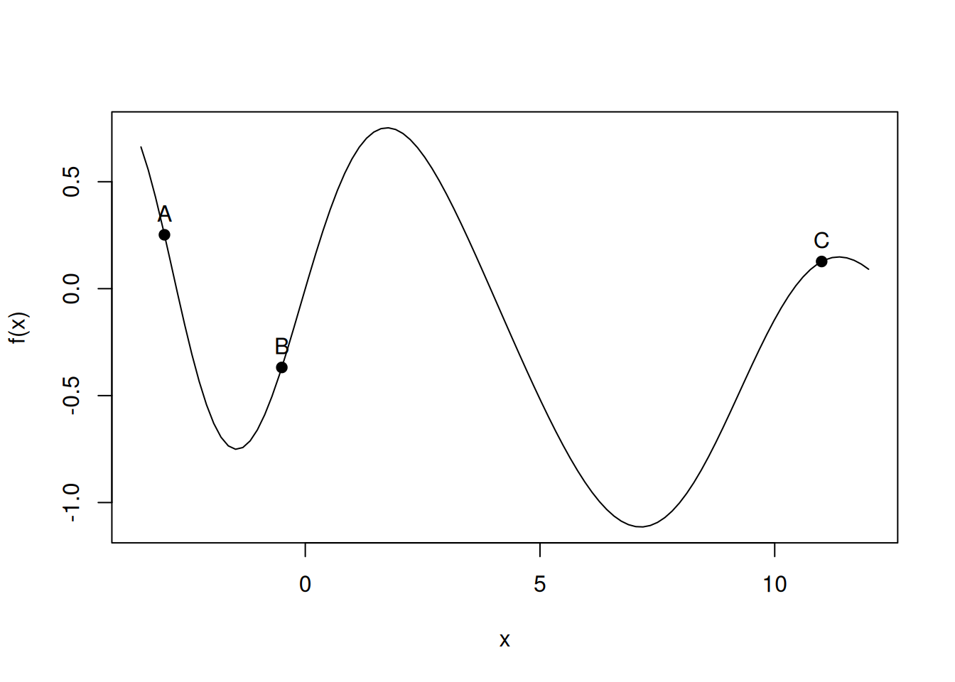
Figure 4.1: \(f(x) = \sin{(x-0.04x^2)} - \frac{\sin{(x)}}{4}\)
The easier way to find the solution is by the Bracketing method. We first need to find three points, \(A\), \(B\) and \(C\), such that \(f(A)>f(B)\) and \(f(C)>f(B)\) as in Figure 4.1. The following function computes the solution using the Algorithm 4.1 of Judd (1998) (I also create a print method. Why not keeping our good habits):
Brack <- function(f,a,b,c,eps=1e-8,maxit=1000)
{
if (f(a)<=f(b) | f(c)<=f(b))
  stop("You must have f(a), f(c) > f(b)")
if (!(b<c) | !(b>a) )
    stop("You must have a<b<c")
crit=1000; n <- 1; x <- c(a,b,c)
mess <- NULL
conv <- T
id <- 0
fb <- f(b)
while(TRUE)
    {
    d <- ifelse((b-a)<(c-b),(c+b)/2,(b+a)/2)
    fd <- f(d)
    if (d<b & fd>fb)
    {
      a <- d
  } else if (d<b & fd<fb) {
        c<-b
        b<-d
        fb <- f(b)
    } else if(d>b & fd<fb) {
        a<-b
        b<-d
        fb <- f(b)
    } else {
        c <- d
    }
    crit <- c-a
    x <- rbind(x,c(a,b,c))
    if (n>=maxit){
        mess <- paste("maxit(",maxit,") reached",sep="")
        conv=F
        break}
    n <- n+1
    if (crit < eps*abs(b))
        break
    }
n <- nrow(x)
ans <- list(obj=f(b),x=x,sol=b,name="Bracketing Method",conv=conv,prec=(x[n,3]-x[n,1]),mess=mess)
class(ans) <- "NonlinSol"
return(ans)
}
print.NonlinSol <- function(obj)
    {
    n <- nrow(obj$x)
    cat("\nMethod: ",obj$name,"\n")
    if (obj$conv)
        cat("Message: Converged after ",(n-1)," iterations", obj$mess,"\n\n")
    else
        cat("Message: ",obj$mess,"\n\n")
    if(length(obj$sol)==1)
        cat("The solution is: ",obj$sol,", and f(x) is ",obj$obj,"\n")
    else
        {
        cat("The solution is: \n")
        if(is.null(names(obj$sol)))
            names(obj$sol) <- paste("x",1:length(obj$sol),sep="")
        for(i in 1:length(obj$sol))
            cat(names(obj$sol)[i]," = ",obj$sol[i],"\n")
        cat("\nf(x) is ",obj$obj,"\n")
        }
    cat("Precision: ",obj$prec,"\n")
    }
Before we solve the problem, we have to ask ourselves: how should we pick the \(\epsilon\)? We know that the solution is between \(a\) and \(c\). Therefore, should we make it as small as possible? This is a very good application of floating-point arithmetic that we covered in Chapter 2. Suppose that the true solution is \(b\) (see Press et al. (2007), Chapter 10). Then, a Taylor approximation implies (remember that the first derivative is zero at that point): \[ f(x) \approx f(b) + \frac{1}{2}f''(b)(x-b)^2 = f(b) \left( 1 + \frac{f''(b)(x-b)^2}{2f(b)}\right) \] The last term will be numerically equal to \(f(b)\) whenever: \[ \frac{f''(b)(x-b)^2}{2|f(b)|} <\epsilon_m , \] where \(\epsilon_m\) is the machine epsilon. Remember that by definition \((1+\epsilon_m)=1\) numerically. It implies that: \[ |x-b| < \sqrt{\epsilon_m}\sqrt{\frac{2|f(b)|}{f''(b)}} = \sqrt{\epsilon_m}|b|\sqrt{\frac{2|f(b)|}{b^2f''(b)}} = \sqrt{\epsilon_m}|b| O(1) \] The moral is that there is no point of making the interval \([a,c]\) smaller than \(\sqrt{\epsilon_m}|b|\) because we would not see any difference in terms of function values. For example, if the middle point is 1, then setting the tolerance level to \(10^{-8}\) is the best we can do. With the three points shown in Figure 4.1, the solution is:
##
## Method:  Bracketing Method
## Message: Converged after  47  iterations
##
## The solution is:  7.143987 , and f(x) is  -1.114449
## Precision:  6.426126e-08
plotBack <- function(f,a,b,c,n,from,to)
{
res <- Brack2(f,a,b,c)
x <- res$x[1:n,]
pres <- curve(f,from,to,ylab="f(x)",xlab="x",
main="The convergence of the Bracketing Method")
os <- (max(pres$y)-min(pres$y))*1.5/30
points(c(a,b,c),f(c(a,b,c)),pch=21,bg=1)
text(a,f(a)+os,"A")
text(b,f(b)+os,"B")
text(c,f(c)+os,"C")
n <- min(nrow(res$x),n)
for (i in 2:n)
{
w <- which(x[(i-1),]!=x[i,])
l <- apply(as.matrix(x[i,]),1,function(s) sum(x[1:(i-1),]==s))+1
xi1 <- x[(i-1),w]; xi <- x[i,w]
fi1 <- f(xi1); fi <- f(xi)
text(x[i,1],f(x[i,1])+os*l[1],"A",col=i,lwd=2)
text(x[i,2],f(x[i,2])+os*l[2],"B",col=i,lwd=2)
text(x[i,3],f(x[i,3])+os*l[3],"C",col=i,lwd=2)
points(xi,fi,pch=21,bg=i)
for (j in 1:sum(w))
arrows(xi1[j],fi1[j],xi[j],fi[j],col=i,lty=2,lwd=2)
}
}We can see how the algorithm works by looking at Figures 4.2 and 4.3. In the first one, we reach the global minimum and in the second we only find a local one. The result from the second set of starting values is:
##
## Method:  Bracketing Method
## Message: Converged after  47  iterations
##
## The solution is:  -1.460872 , and f(x) is  -0.7512074
## Precision:  9.313226e-09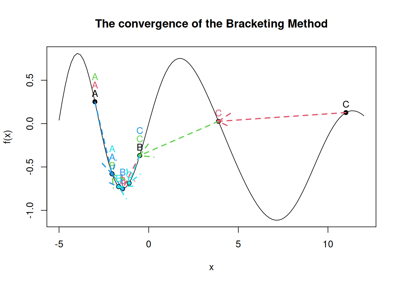
Figure 4.2: \(f(x) = \sin{(x-0.04x^2)} - \frac{\sin{(x)}}{4}\)
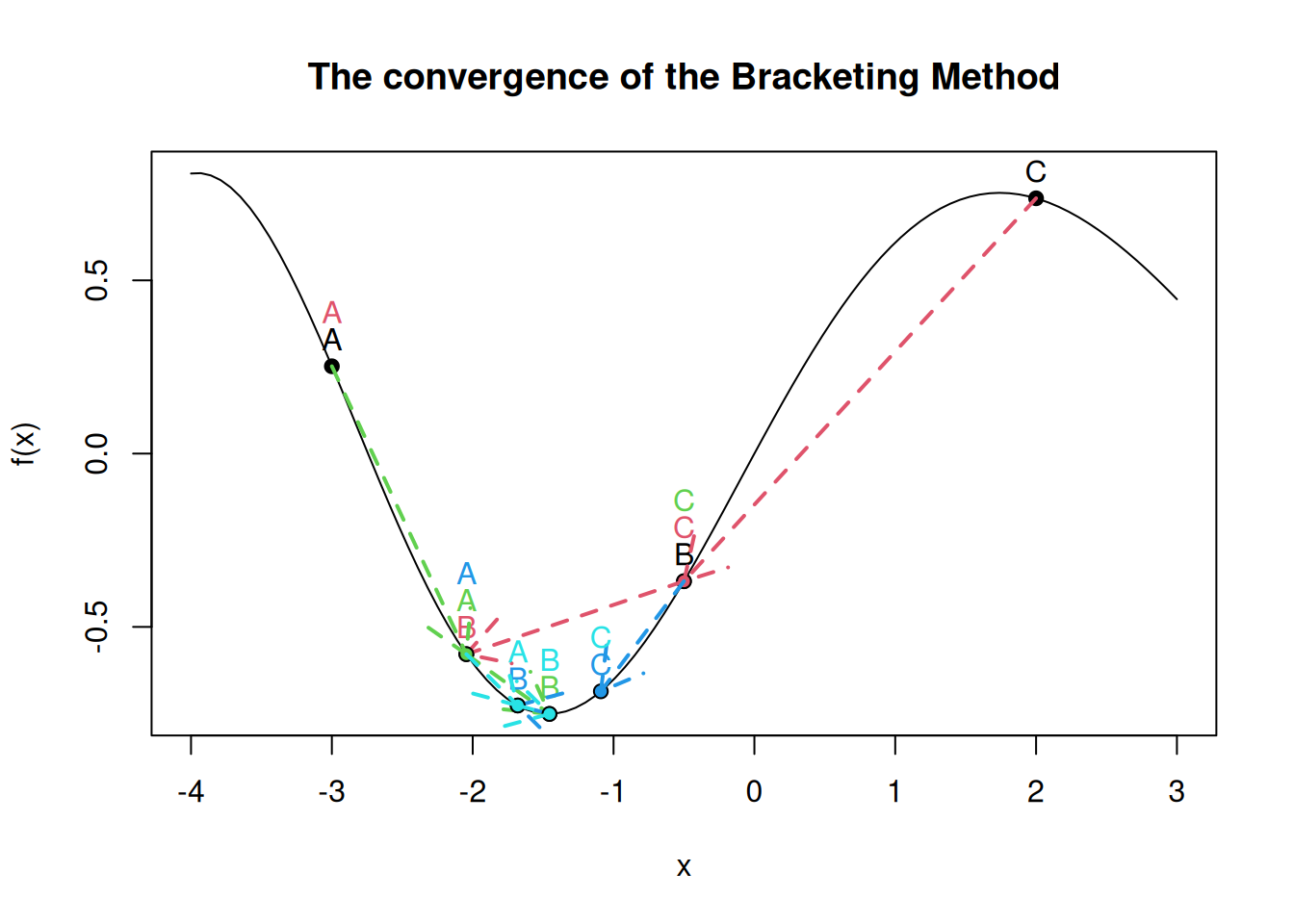
Figure 4.3: \(f(x) = \sin{(x-0.04x^2)} - \frac{\sin{(x)}}{4}\) (Different starting points)
The above method is not the most efficient one. The method put the fourth point in the middle of the largest interval between \([a,b]\) and \([b,c]\). We can improve the number of iterations by selecting another fraction. The Golden Section proceeds as follows: if \((b-a)>(c-b)\), then \(d=b-\delta(c-a)\) and if \((b-a)<(c-b)\), then \(d=a+\delta(c-a)\), where \(\delta=(3-\sqrt{5})/2\). Assume that \(b=a + \delta(c-a)\), which forms the original three points, and the fourth point \(d\) is \(b+\omega(c-a)\).
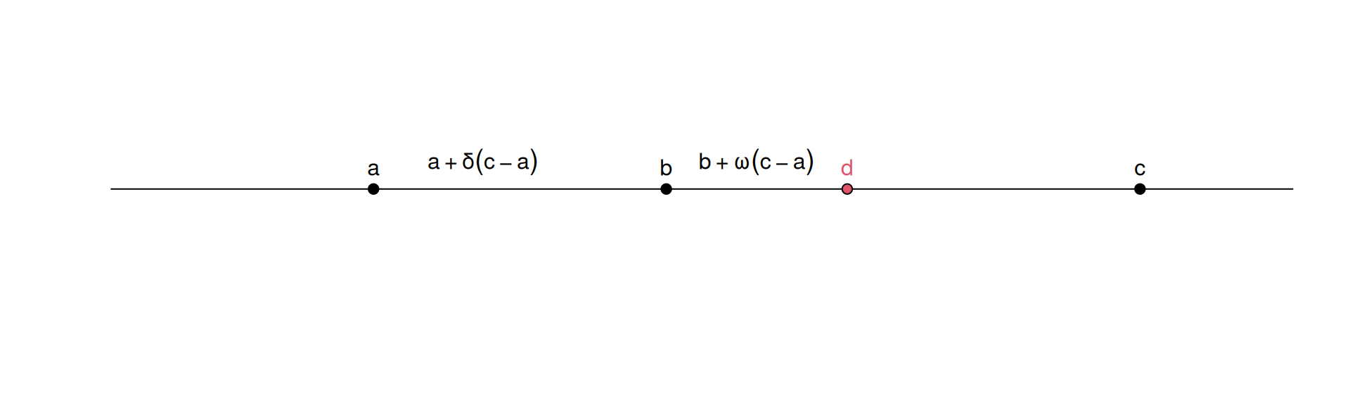
Since we either pick \(\{a,b,d\}\) or \(\{b,d,c\}\) the relative length is either: \[ \frac{d-a}{c-a} = \omega+\delta \] or \[ \frac{c-b}{c-a} = 1-\delta \] We minimize the worse scenario by making it equal to the best one. In other words, we set \((\omega+\delta)=(1-\delta)\) or \(\omega=(1-2\delta)\). Also, we assume, like for \(d\), that \(b\) was optimal so that \((b-a)/(c-a)=(d-b)/(c-b)\) which implies: \[ \delta = \frac{d-b}{c-b} = \frac{\omega(c-a)}{c-b} = \omega(1-\delta) \] If we combine \(\delta(1-\delta)=\omega\) and \(\omega=(1-2\delta)\), we get a second order polynomial with the only positive solution being \((3-\sqrt{5})/2\). The following uses the optimal ratio:
##
## Method:  Bracketing Method
## Message: Converged after  39  iterations
##
## The solution is:  -1.460872 , and f(x) is  -0.7512074
## Precision:  2.860287e-08
It is better, but not that much better. The algorithm has a linear convergence. There exists a super-linear method for one dimensional problems. It is the Brent’s method. It only defers in the way the fourth point is selected.
4.1.2 Methods based on Derivatives
A method that only requires one staring point is the Newton’s Method. It is based on the Taylor approximation of \(f(x)\): \[ p(x) = f(a) + f'(a)(x-a) + \frac{f''(a)}{2}(x-a)^2 \] The solution of the minimization problem is: \[ x^* = a - \frac{f'(a)}{f''(a)} \] We can therefore build our iterative scheme based on the solution: \[ x_{k+1} = x_k - \frac{f'(x_k)}{f''(x_k} \] The problem here is that we need the first and second derivative. The function I am proposing is a general function that requires \(f\) to be an expression so that we can obtain the derivatives using D():
Newton <- function(f,x0,eps=1e-8,delta=1e-8,maxit=1000)
    {
    go <- TRUE; n <- 1
    mess <- NULL
    res <- c(x0,eval(f,list(x=x0)))
    Df <- D(f,"x")
    DDf <- D(Df,"x")
    conv <- T
    while (go)
        {
        x <- x0 - eval(Df,list(x=x0))/eval(DDf,list(x=x0))
        crit1 <- abs(x-x0)/(1+abs(x0))
        crit2 <- abs(eval(Df,list(x=x0)))
        go <- !(crit1<eps & crit2<delta)
        res <- rbind(res,c(x,eval(f,list(x=x))))
        if (n>=maxit)
            {
            mess <- paste("maxit(",maxit,") reached",sep="")
            conv <- FALSE
            break
            }
        x0 <- x
        n <- n+1
        }
if (eval(DDf,list(x=x0))<=0)
    mess2 <- "not satisfied"
else
    mess2 <- "satisfied"
mess <- paste(mess," (SOC ",mess2,")",sep="")
n <- nrow(res)
ans <- list(obj=res[n,2],sol=x,x=res,name="Newton's Method",conv=conv,prec=crit1,mess=mess)
class(ans) <- "NonlinSol"
return(ans)
}
We can try the function using the example we use above. We see that the method just finds stationary points. It could be a maximum or a minimum. We can see what happens if we start at 10 and 8.5:
##
## Method:  Newton's Method
## Message: Converged after  6  iterations  (SOC not satisfied)
##
## The solution is:  11.36565 , and f(x) is  0.1485208
## Precision: 7.757233e-15##
## Method: Newton's Method
## Message: Converged after 5 iterations (SOC satisfied)
##
## The solution is: 7.143987 , and f(x) is -1.114449
## Precision: 3.667952e-10By the number of iterations, it is much faster than the Bracketing Method. However, it is very sensitive to starting values when we have multiple extrema. Figure 4.4 shows the details of some iterations and different starting values (the functions for plotting the convergence of the the Bracketing and Newton’s methods are available in the .R file of Chapter 4 on the website of the course).
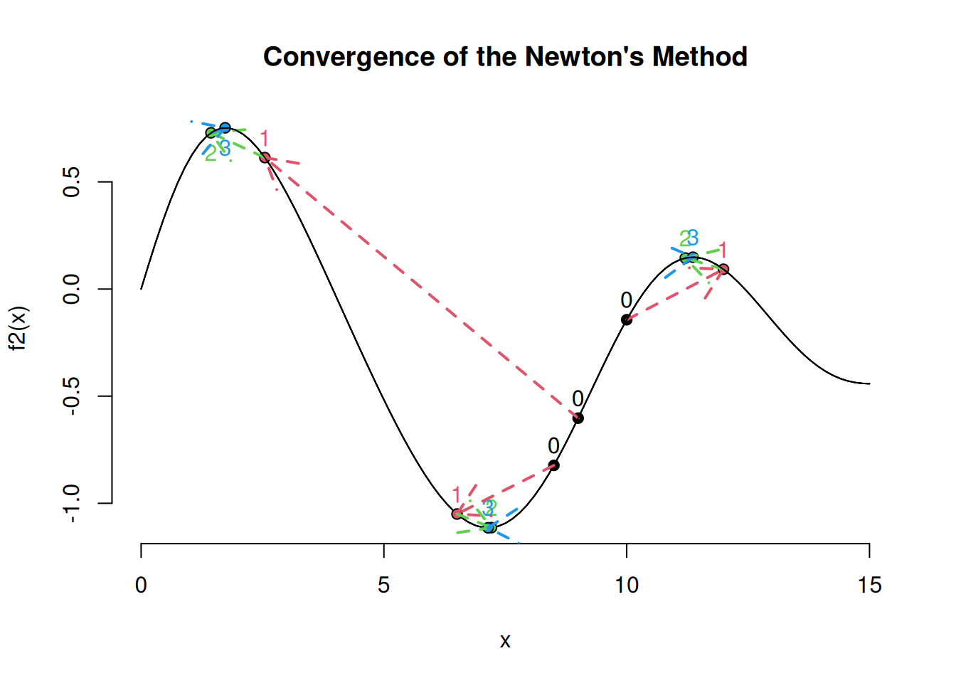
Figure 4.4: \(f(x) = \sin{(x-0.04x^2)} - \frac{\sin{(x)}}{4}\) (Newton Method)
If we look at the example page 98 of Judd (1998), we want to maximize the utility function: \[ U = x^{1/2} + 2y^{1/2} \] subject to the constraint \(2x+3y=1\). We can solve this problem by substitution. By doing it, the problem is reduced to a one dimensional optimization problem: \[ U = \left(\frac{1-3y}{2}\right)^{1/2} + 2 y ^{1/2} \] The solution must be between 0 and 1/3, so we can try the triplet (0,1/6,1/3) for the Bracketing method and a starting value of .1 for the Newton’s method (we have to return the negative of the utility because we have developed minimization algorithms). Figures 4.5 and 4.6 show the details of the convergence.
f <- function(x) -((1-3*x)/2)^.5-2*x^.5
f2 <- expression(-((1-3*x)/2)^.5-2*x^.5)
resB <- Brack(f,0,1/6,1/3)
resN <- Newton(f2,.1)
resB
##
## Method: Bracketing Method
## Message: Converged after 47 iterations
##
## The solution is: 0.2424242 , and f(x) is -1.354006
## Precision: 1.241763e-09##
## Method: Newton's Method
## Message: Converged after 6 iterations (SOC satisfied)
##
## The solution is: 0.2424242 , and f(x) is -1.354006
## Precision: 1.268904e-14## [1] 0.1363636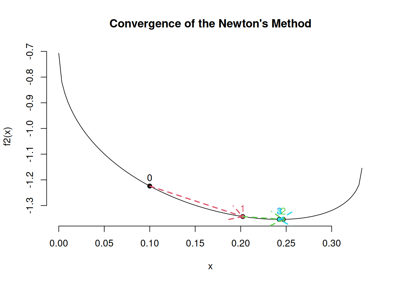
Figure 4.5: Minimization of \(-U = -x^{1/2}-2y^{1/2}\), with \(x=(1-3y)/2\) (The Newton Method)
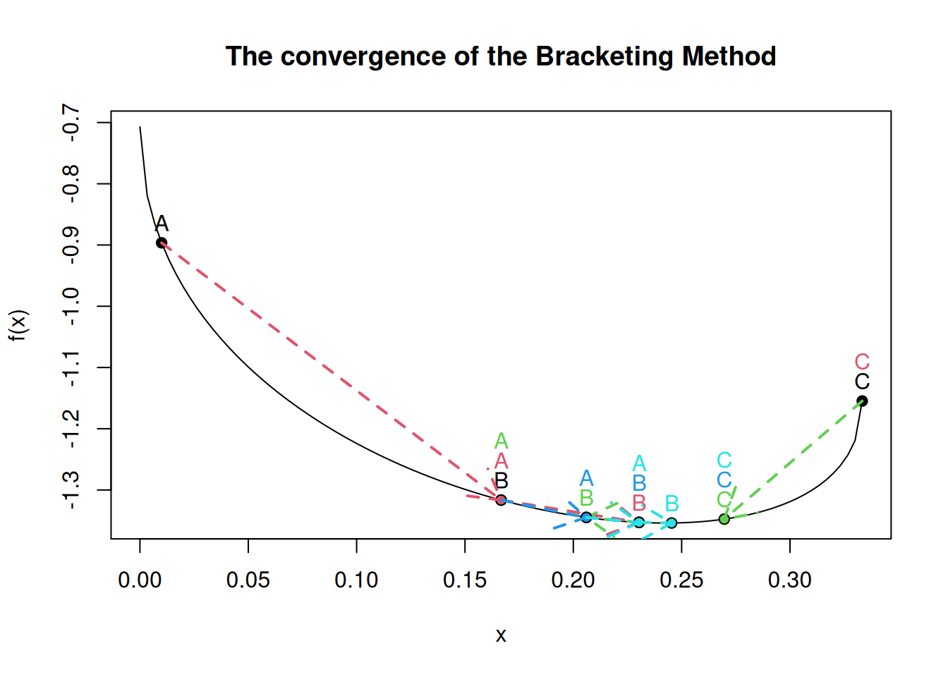
Figure 4.6: Minimization of \(-U = -x^{1/2}-2y^{1/2}\), with \(x=(1-3y)/2\) (The Bracketing Method)
Suppose we want to solve the consumer problem: \[ \max_{x,y} -e^{-x}-e^{-y} \] subject to \[ 2x+3y=10000 \] which implies the following unconstrained problem \[ \max_{y} -e^{-5000+1.5y}-e^{-y} \]
##
## Method:  Newton's Method
## Message:  maxit(600) reached (SOC satisfied)
##
## The solution is:  700 , and f(x) is  9.859677e-305
## Precision:  0.001428571
This is a case of scaling problem. The algorithm reached at some point the zero (underflow), which result in a failure (if we don’t restrict the number of iterations). One solution to this problem is to rewrite the problem as: \[ y-x=\log{(2/3)} \] \[ 2x+3y=10000 \] And solve it using matrix algebra:
## [1] 2000.243 1999.8384.2 Multidimensional Optimization
4.2.1 A monopoly problem
Consider the problem in which a monopoly maximizes the following profit function: \[ \Pi(Y,Z) = P_y(Y,Z)Y + P_z(Y,Z)Z - C_y(Y)-C_z(Z) \] where the inverse demands \(P_y(Y,Z)\) and \(P_z(Y,Z)\) are derived from the utility function: \[ \begin{split} U = & (Y^\alpha+Z^\alpha)^{\eta/\alpha} + M\\ = & u(Y,Z) + M \end{split} \] where \(M\) is the dollar expenditure on other goods. In other words, the consumer’s problem is: \[ \max_{Y,Z} u(Y,Z) + (I-P_zZ-P_yY), \] where \(I\) is the consumer’s income. It implies that \(P_y(Y,Z) = u_y(Y,Z)\) and \(P_z(Y,Z)=u_z(Y,Z)\). The monopoly problem is therefore: \[ \max_{Y,Z} u_y(Y,Z)Y + u_z(Y,Z)Z - C_y(Y)-C_z(Z), \] where, \(C_y(Y)=0.62Y\), \(C_z(Z)=0.60Z\), \(\alpha=0.98\), and \(\eta=0.85\). In the book, the author suggests to redefine the variables \(Y\) and \(Z\) to allow the admissible space to be the real line. Because \(\alpha\) is less than one, \(Y\) and \(Z\) cannot be negative. Such restrictions may create problems. So we will solve for \(y=\log{Y}\) and \(z=\log{Z}\) instead. The function is
Profit <- function(y,z)
{
  Y=exp(y)
  Z=exp(z)
  a=0.98
  n=0.85
  A=n*(Y^a+Z^a)^(n/a-1)
  R = A*(Y^a+Z^a)-0.62*Y-0.60*Z
  return(-R)
}
There are two ways to see the shape of a three dimensional function in R. You can use the contour or the wireframe from the Sarkar (2026) package. For the latter, I am not transforming the variable because it makes the function look flat. It is easier that way to see the shape. The solution of the problem is \(y=-0.562\) (or \(Y=0.57\)) and \(z=1.077\) (or \(Z=2.936\)).
y <- seq(-1.5,0,length=200)
z <- seq(0.5,1.5,length=200)
x <- outer(y,z,Profit)
contour(x=y,y=z,z=x,nlevels=20,xlab="log(Y)",ylab="log(Z)")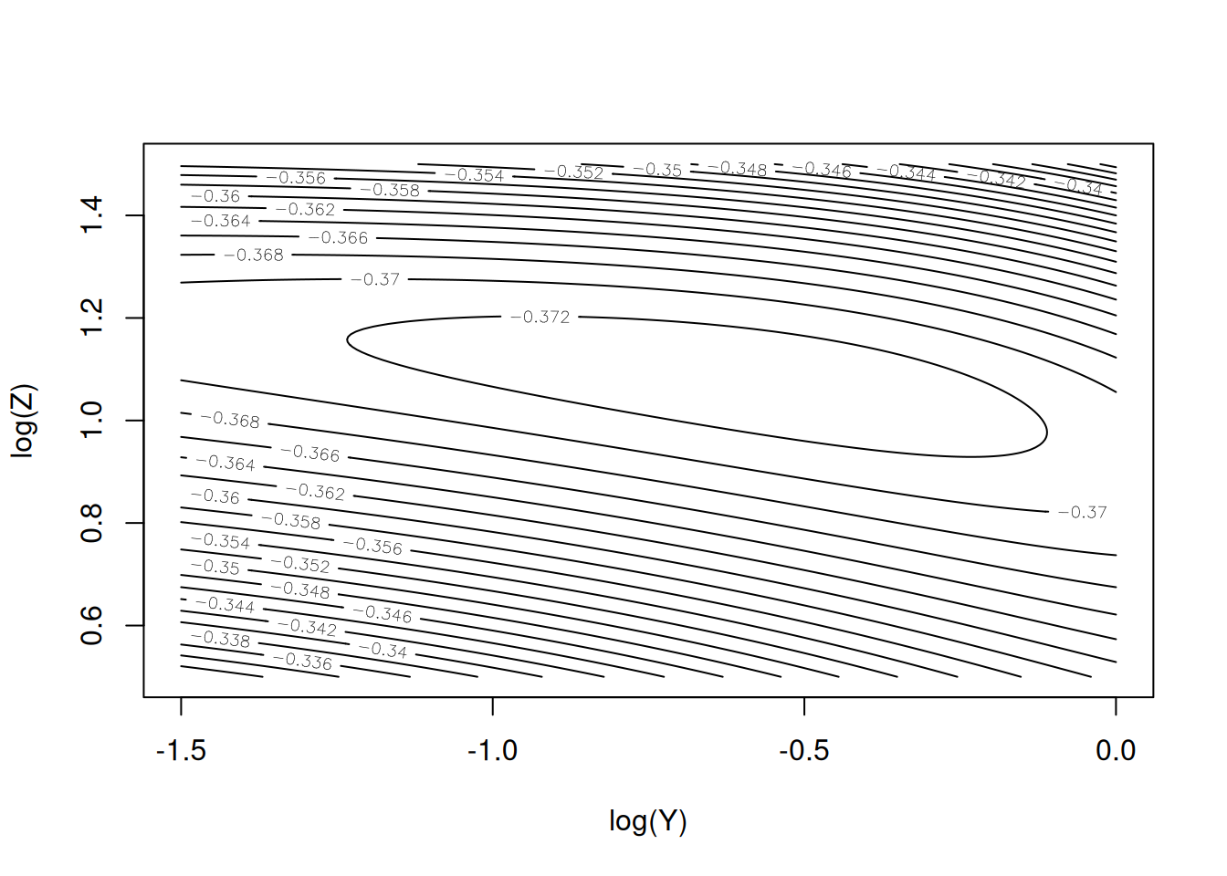
library(lattice)
Profit2 <- function(Y,Z)
{
  a <- 0.98; n <- 0.85
  A=n*(Y^a+Z^a)^(n/a-1)
  R = A*(Y^a+Z^a)-0.62*Y-0.60*Z
  return(-R)
}
z <- seq(2,4,length=50)
y <- seq(0,2,length=50)
res <- expand.grid(y,z)
x <- Profit2(y<-res$Var1,z<-res$Var2)print(wireframe(x~y*z ,xlab="Y",ylab="Z",zlab="Profit",
scales = list(arrows = FALSE), drape = TRUE, colorkey = TRUE))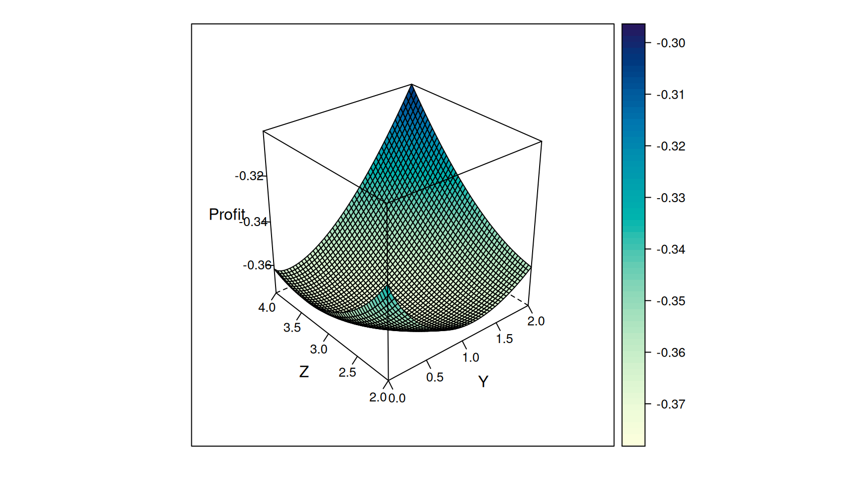
Exercise 4.1 Build an algorithm that finds the minimum of a function using the Grid Search method. The function will be: Grid(f,from, to, n, eps), where \(f\) is a function of \(x\), a \(k\times 1\) vector, from and to are the lower and upper bounds of \(x\), n is the number of points per variable, and eps if the tolerance level. Test your function using the above example.
4.2.2 Newton’s Method
The first method is the Newton’s Method. It is the multidimensional version of the one presented in Section 4.1.2. The procedure is: \[ x_{k+1} = x_k - H(x_k)^{-1}J(x_k), \] where \(J()\) is the Jacobian and \(H()\) the Hessian of the function we are minimizing. If \(f()\) is an expression, it is easy to build the algorithm:
getDer <- function(f,x)
{
    # x must contain the names of the variables
    n <- length(x)
    x <- as.list(x)
    J <- vector()
    H <- matrix(0,n,n)
    for (i in 1:n)
        {
        Df <- D(f,names(x[i]))
        J[i] <- eval(Df,x)
        for(j in 1:i)
            H[i,j] <- eval(D(Df,names(x[j])),x)
        }
    H[upper.tri(H)]<-H[lower.tri(H)]
    dimnames(H) <- list(names(x),names(x))
    names(J) <- names(x)
    return(list(H=H,J=J))
}

MNewton <- function(f,x0,eps=1e-8,delta=1e-8,maxit=1000)
{
    n <- 1
    conv=TRUE
    mess <- NULL
    fx <- eval(f,as.list(x0))
    res <- c(x0,fx)
    while(TRUE)
    {
        resD <- getDer(f,x0)
        H <- resD$H
        J <- resD$J
        x <- x0 - solve(H,J)
        fx <- eval(f,as.list(x))
        res <- rbind(res,c(x,fx))
        crit1 <- sqrt(crossprod(x-x0))/(1+sqrt(crossprod(x0)))
        if (crit1<eps)
        {
            crit2 <- sqrt(crossprod(J))/(1+abs(fx))
            if (crit2<delta)
                break
        }
        if(n>=maxit)
        {
            mess <- paste("maxit(",maxit,") reached",sep="")
            conv=FALSE
            break
        }
        x0 <- x
        n <- n+1
    }
  n <- nrow(res)
  ans <- list(obj=res[n,ncol(res)],sol=x,x=res,name="Newton's Method for Multidimensional Problems",conv=conv,prec=crit1,mess=mess)
  class(ans) <- "NonlinSol"
  return(ans)
}
We can then try it with the monopoly problem, and plot the result on a contour plot:
f <- expression(-0.85*(exp(y)^0.98+exp(z)^0.98)^(0.85/0.98-1)*(exp(y)^0.98 +
    exp(z)^0.98)+0.62*exp(y)+0.6*exp(z))
res <- MNewton(f,c(y=1,z=1))
res
##
## Method: Newton's Method for Multidimensional Problems
## Message: Converged after 9 iterations
##
## The solution is:
## y = -0.5625466
## z = 1.076945
##
## f(x) is -0.3731764
## Precision: 3.098286e-15y <- seq(-1,1.5,length=200)
z <- seq(0,2,length=200)
x <- outer(y,z,Profit)
contour(x=y,y=z,z=x,nlevels=20,xlab="log(Y)",ylab="log(Z)")
text(res$x[1:6,1],res$x[1:6,2]+.1,c("A","B","C","D","E","F"))
points(res$x[1:6,1],res$x[1:6,2],pch=21,bg=2)
lines(res$x[1:6,1],res$x[1:6,2],col=4)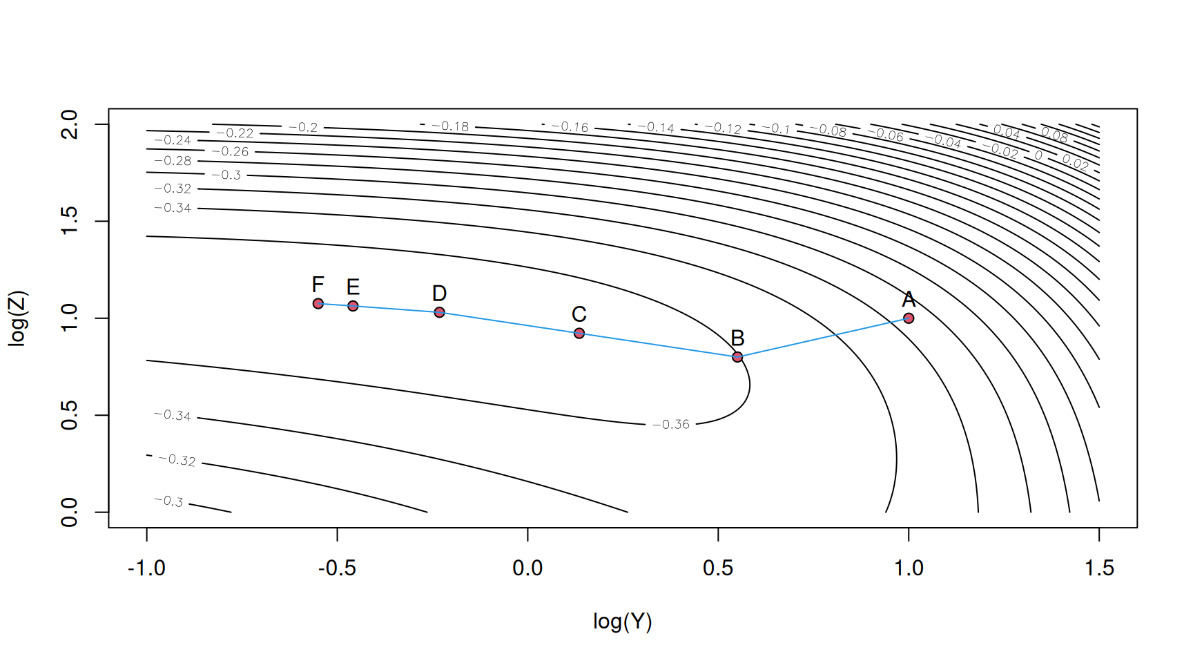
As for the unidimensional case, the method works well when we start not too far from the solution or if the function is well behaved. For the monopoly problem, we reach the solution using almost any starting values.
##
## Method:  Newton's Method for Multidimensional Problems
## Message: Converged after  14  iterations
##
## The solution is:
## y  =  -0.5625466
## z  =  1.076945
##
## f(x) is  -0.3731764
## Precision: 1.365248e-14##
## Method: Newton's Method for Multidimensional Problems
## Message: Converged after 22 iterations
##
## The solution is:
## y = -0.5625466
## z = 1.076945
##
## f(x) is -0.3731764
## Precision: 4.912394e-09Exercise 4.2 Write a function that combines the Newton’s and the Grid Search methods. It must use the grid search function you built for Exercise @ref{exr:optim1} to find a starting vector. The latter is then, use to initiate the Newton’s Method. Try it with the monopoly problem.
4.2.3 Direction Set Methods
Most optimization algorithms in R or any other numerical software are Direction Set Methods. The general step is \[ x_{k+1} = x_k + \lambda_k s_k, \] where \(s_k\) is a vector representing the search direction and \(\lambda_k\) is a scalar. All methods differ in their respective choice of the search direction \(s_k\). On the other hand, the method for computing \(\lambda_k\) is identical. If we want to minimize \(f(x)\), \(\lambda_k\) is defined as: \[ \lambda_k = \arg \min_\lambda f(x_k + \lambda s_k) \]
Exercise 4.3 Write a function that compute \(\lambda_k\). The function must have the form: getLambda(f,x,s), where \(f\) is either an expression or a function (it is up to you). You can also allow the two possibilities. You can verify your function by using the Profit function. You should get (The function is hidden from the notes):
## [1] -1.378165We can summarize the different methods as follows (we consider the problem of minimizing \(f(x)\), with \(x \in \mathbb{R} ^n\):
- Coordinate Direction: \(s_k = e_i\) for \(i=1,...,n\) for each iteration (\(n\) directions by iteration), where \(e_i\) is the \(n\times 1\) vector with the \(i^{th}\) element equals to 1 and all others being equal to zero. (Always find a minimum when the function is smooth but may be slow)
- Steepest Descent: \(s_k = -J(x_k)\) (Always find a minimum when the function is smooth but may be slow)
- Newton’s Method with Line Search: \(s_k=-H(x_k)^{-1}J(x_k)\). As opposed to the Newton’s Method, it will always go downhill.
- Broyden-Fletcher-Goldfarb-Shanno (BFGS): \(s_k=-H(x_k)^{-1}J(x_k)\), but \(H_k\) is just an approximation of the hessian matrix. Starting with \(H_0=I\), the updates are: \[H_{k+1} = H_k - \frac{H_kz_kz_k'H_k}{z_k'H_kz_k} + \frac{y_ky_k'}{y_k'z_k}\], where \(z_k=x_{k+1}-x_k\) and \(y_k=J(x_{k+1})-J(x_k)\). Whenever, \(y_k'z_k\approx 0\), \(H_{k+1}=H_k\).
- Conjugate Gradient: This method does not require the Hessian matrix; only the Jacobian. The steps are: \(s_0=-J(x_0)\) and \[s_{k+1} = -J(x_{k+1})+\frac{\|J(x_{k+1})\|^2}{\|J(x_{k})\|^2}s_k\] and reset \(s_k\) to \(-J(x_{k})\) every \(n\) iterations.
- Gauss-Newton Method for Nonlinear Least Squares: This method is specific to the following problem: \[f(x) = \sum_{i=1}^{T} e_i^2(x)\], where \(e_i(x)\) is the \(i^{th}\) residual (here, \(x\) is the vector of coefficients). Let the \(T\times n\) matrix \(J(x)\) be the Jacobian of the vector of residuals \(e(x)\). Than the Gauss-Newton step is: \[s_k = -[J(x_k)'J(x_k)]^{-1}[J(x_k)'e(x_k)]\]. It is like the Newton’s Method but the Hessian is approximated by \([J(x_k)'J(x_k)]\).
We first consider an application of the Gauss-Newton method. Lets consider the following Box-Cox transformation: \[ \frac{y_i^\lambda-1}{\lambda} = \alpha + \beta z_i + e_i \] The vector \(x\) is \(\{\lambda,\alpha,\beta\}\). The \(i^{th}\) line of \(J\) is then: \[ J(x)[i,] = \frac{\partial e_i}{\partial x} = \begin{pmatrix} \frac{y_i^\lambda [\lambda \log{(y_i)}-1] +1}{\lambda^2} & -1 & -z_i \end{pmatrix} \] The following function applies the method but without line search:
GaussNewton <- function(f,x0,dat,eps=1e-8,delta=1e-8,maxit=1000)
{
    # f produces the vector of residuals
    # dat must be a list, x0 a named vector
    Jfct <- function(x,dat)
    {
      J <- eval(D(f,names(x)[1]),c(as.list(x),dat))
        for(i in 2:length(x))
            J <- cbind(J,eval(D(f,names(x)[i]),c(as.list(x),dat)))
        return(J)
    }
  n <- 1;   conv=TRUE; mess <- NULL
    fx <- eval(f,c(as.list(x0),dat))
    res <- c(x0,sum(fx^2))
    while(TRUE)
    {
      J <- Jfct(x0,dat)
        H <- crossprod(J)
        J <- crossprod(J,fx)
        x <- c(x0 -solve(H,J))
        names(x) <- names(x0)
        fx <- eval(f,c(as.list(x),dat))
        res <- rbind(res,c(x,sum(fx^2)))
        crit1 <- c(sqrt(crossprod(x-x0))/(1+sqrt(crossprod(x0))))
        if (crit1<eps)
        {
            crit2 <- c(sqrt(crossprod(J)))/(1+sum(fx^2))
            if (crit2<delta)
                break
        }
        if(n>=maxit)
        {
            mess <- paste("maxit(",maxit,") reached",sep="")
            conv=FALSE
            break
        }
        x0 <- x
        n <- n+1
    }
  n <- nrow(res)
  ans <- list(obj=res[n,2],sol=x,x=res,name="Gauss-Newton's Method for NLS Problems",conv=conv,prec=crit1,mess=mess)
  class(ans) <- "NonlinSol"
  return(ans)
}
We can see that the method does not work well for the Box-Cox estimation. Even if we try different starting values, the algorithm diverges. The problem is that the approximated Hessian becomes singular.
f <- expression((y^l-1)/l -a -z*b)
library(Ecdat, quietly = TRUE)
data(Consumption)
C <- Consumption[,"ce"]
z <- ts(1:length(C),freq=4,start=c(1947,1))
dat <- list(y=C,z=z)
res2 <- try(GaussNewton(f,c(l=.25,a=56,b=.2),dat,maxit=50,eps=1e-4))
## Error in solve.default(H, J) :
## system is computationally singular: reciprocal condition number = 1.11394e-16## Error in solve.default(H, J) :
## system is computationally singular: reciprocal condition number = 1.11394e-16In some cases, however, it works fine. Consider the following nonlinear model: \[ Y_i = \alpha_1 + \alpha_2\alpha_3x_i+\alpha_2^2z_i + \epsilon_i \] In the following, I test the method using simulated data with \(\alpha_1=2\), \(\alpha_2=3\), and \(\alpha_3=5\). We can see that the method works fine.
x <- rnorm(200)
z <- rnorm(200)
y <- 2+3*5*x+9*z+rnorm(200)
f <- expression(y-a1-a2*a3*x-a2^2*z)
dat <- list(y=y,x=x,z=z)
x0 <- c(a1=0,a2=1,a3=1)
res3 <- try(GaussNewton(f,x0,dat,maxit=100))
print(res3)
##
## Method: Gauss-Newton's Method for NLS Problems
## Message: Converged after 7 iterations
##
## The solution is:
## a1 = 1.924971
## a2 = 3.006015
## a3 = 4.970117
##
## f(x) is 3.006015
## Precision: 6.237973e-17Exercise 4.4 Reproduce the results from Table 4.12 (Section 4.11) of Judd (1998). You have to compare the Newton and Gauss-Newton Methods for the following model: \[ y=\alpha x_1 + \beta x_2 + \beta^2 x_3 + \epsilon \] The residual sum of squares is: \[ \begin{split} S(\alpha,\beta) =& 38.5-5.24\alpha-7.56 \alpha^2-6.10\beta+9.96\alpha\beta\\ & - 3.44\beta^2+11.4\alpha\beta^2+11.6\beta^3+7.71\beta^4 \end{split} \]
I conclude the section with a function to compute the BFGS method. For that function, I require \(f\) to be a function and we have to provide a function that computes the Jacobian. This setup does not exclude the use of symbolic derivatives. Here is an example using the Box-Cox model:
fBC <- function(beta,dat)
{
    e <- expression((y^l-1)/l-a1-a2*x)
  sum(eval(e,c(as.list(beta),dat))^2)/2
}
DfBC <- function(beta,dat)
{
    e <- expression((y^l-1)/l-a1-a2*x)
    J <- eval(D(e,names(beta)[1]),c(as.list(beta),dat))
    for (i in 2:length(beta))
        J <- cbind(J,eval(D(e,names(beta)[i]),c(as.list(beta),dat)))
    et <- eval(e,c(as.list(beta),dat))
    crossprod(J,et)
}
To allow both the case of theoretical and empirical models, The ... can be passed to \(f\) and \(grad\) when we need to use data or set other parameter values.
BFGS <- function(f,x0,grad,eps=1e-8,delta=1e-8,maxit=100,...)
{
    n <- 1
    conv=TRUE
    mess <- NULL
    fx <- f(x0, ...)
    res <- c(x0,fx)
    H <- diag(length(x0))
    while(TRUE)
    {
        J <- grad(x0,...)
        s <- solve(H,-J)
        l <- getLambda(f,x0,s,-50,50,...)
        x <- x0 +l*s
        names(x) <- names(x0)
        fx <- f(x, ...)
        res <- rbind(res,c(x,fx))
        crit1 <- sqrt(crossprod(x-x0))/(1+sqrt(crossprod(x0)))
        if (crit1<eps)
        {
            crit2 <- sqrt(crossprod(J))/(1+abs(fx))
            if (crit2<delta) break
        }
        if(n>=maxit)
        {
            mess <- paste("maxit(",maxit,") reached",sep="")
            conv=FALSE; break
        }
        zk <- (x-x0); yk <- J-grad(x,...)
        T1 <- c(t(yk)%*%zk)
        T2 <- H%*%zk%*%t(zk)%*%H
        T3 <- c(t(zk)%*%H%*%zk)
        if (abs(T1) > 1e-7)
            H <- H - T2/T3 + (yk%*%t(yk))/T1
        n <- n+1
        x0 <- x
    }
  n <- nrow(res)
  ans <- list(obj=res[n,2],sol=x,x=res,name="BFGS Method",conv=conv,prec=crit1,mess=mess)
  class(ans) <- "NonlinSol"
  return(ans)
}
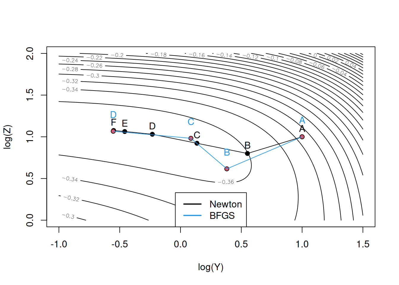
Lets try it on the monopoly problem:
f <- function(x)
{
    fexp <-  expression(-0.85*(exp(y)^0.98+exp(z)^0.98)^(0.85/0.98-1)*(exp(y)^0.98 +
    exp(z)^0.98)+0.62*exp(y)+0.6*exp(z))
    eval(fexp,as.list(x))
}
Df <- function(x)
{
    fexp <-  expression(-0.85*(exp(y)^0.98+exp(z)^0.98)^(0.85/0.98-1)*(exp(y)^0.98 +
    exp(z)^0.98)+0.62*exp(y)+0.6*exp(z))
    Df <- vector()
    for (i in 1:length(x))
        Df[i]<-eval(D(fexp,names(x)[i]),as.list(x))
    Df
} ##
## Method: BFGS Method
## Message: Converged after 11 iterations
##
## The solution is:
## y = -0.5625466
## z = 1.076945
##
## f(x) is 1.076945
## Precision: 9.557722e-09The convergence is faster than the Newton’s method. We see why on the next figure
Exercise 4.5 Answer the following questions
a. Write a function that solves optimization problems by the Coordinate Direction with Line Search.
b. Write a function that solves optimization problems by the Steepest Descent with Line Search.
c. Write a function that solves optimization problems by the Newton’s Method with Line Search.
d. Write a function that solves optimization problems by the Conjugate Gradient with Line Search.
e. Using the above monopoly example, Compare the Coordinate Direction, the Steepest Descent, the Newton’s Method with Line Search, the Conjugate Gradient, the BFGS, and the Newton’s Method on a contour plot.
f. Compare your methods with optim (compare the values of the coefficients and the function, and the number of iterations)
Exercise 4.6 Answer question 1 of Chapter 4 of Judd (1998) (but do not use the Polytope method).
Exercise 4.7 Answer question 2 of Chapter 4 of Judd (1998).
4.2.4 Finite Differences
To avoid having to derive the analytical derivatives, it is possible to compute the derivatives using finite differences. The derivatives are: \[ f'(x) = \lim_{h\rightarrow 0}\frac{f(x+h)-f(x)}{h} \] We can approximate the derivatives by: \[ f'(x) \approx \frac{f(x+h)-f(x)}{h} \] for some small \(h\). To be precise, \(h\) should be of order \(\sqrt{\epsilon_f}|x_c|\), where \(\epsilon_f\) is the rounding error from evaluating f(x) and \(x_c\) is \([f(x)/f''(x)]^{1/2}\) (see Press et al. (2007), page 229, for more details). This is meant to minimize the error. However, the following rule works most of the time: \(h=\max(\epsilon_1 |x|,\epsilon_2)\), where \(\epsilon_1\) can be around the square root of the machine-epsilon (\(10^{-8}\)), and \(\epsilon_2\) is a not too small number. The latter is to prevent problems when \(x\) is close to zero. If we set \(\epsilon_2=10^{-4}\), \(h\) will take that value whenever \(|x|<10^4\). The following computes the numerical derivative of any function:
Lets try it for the following functions at \(x=3\): \(f1(x)=exp(x)\), \(f2(x)=log(x)\), \(f3(x)=(x^2-x)\), \(f4(x)=x^3 \sin{(x)}\):
| Estimated derivative | True Derivative | relative error | |
|---|---|---|---|
| f1(x) | 20.08654 | 20.08554 | 0.00005 |
| f2(x) | 0.33333 | 0.33333 | 0.00002 |
| f3(x) | 5.00010 | 5.00000 | 0.00002 |
| f4(x) | -22.92229 | -22.91956 | -0.00012 |
A better precision can be obtained by using the following formula: \[ f'(x) \approx \frac{f(x+h)-f(x-h)}{2h}, \] which requires \(h\) to be of order \(\epsilon_f^{1/3}|x_c|\). Comparing the two methods is left as an exercise.
Exercise 4.8 Write a function that computes the derivative of f(x) using the above formula. Compare it with the first method using the same 4 functions.
Exercise 4.9 Write two functions to compute the Jacobian and the Hessian of \(f(x)\), where \(x\in \mathbb{R} ^n\). Use the second method presented above.
4.3 Constrained optimization
Suppose we want to solve: \[ \max_{x_1,x_2} x_1^{1/3}x_2^{2/3} \] subject to: \[ 3x_1+5x_2=1000 \] In this section, we only look at the Penalty Method. Instead of imposing the constraint we penalize the objective function if it violates it. We can write the model as follows: \[ \max_{x_1,x_2} x_1^{1/3}x_2^{2/3} - P(3x_1+5x_2-1000)^2 \] P is the cost of violating the constraint. We can than apply any method (the true solution is \(x_1=111.11\), and \(x_2=133.33\)):
f <- expression(-x1^(1/3)*x2^(2/3) + 10*(3*x1+5*x2-1000)^2)
x0 <- c(x1=10,x2=10)
MNewton(f,x0,eps=1e-8,delta=1e-8,maxit=1000)
##
## Method: Newton's Method for Multidimensional Problems
## Message: Converged after 5 iterations
##
## The solution is:
## x1 = 111.1118
## x2 = 133.3342
##
## f(x) is -125.4719
## Precision: 1.062379e-10Here, the precision is not valid.w={0,.5,.8,1.1,2,2,2,1.5,1,0} We see that the third decimal is contaminated. To increase the precision, we need to increase P.
f <- expression(-x1^(1/3)*x2^(2/3) + 10^3*(3*x1+5*x2-1000)^2)
MNewton(f,x0,eps=1e-8,delta=1e-8,maxit=1000)
##
## Method: Newton's Method for Multidimensional Problems
## Message: Converged after 5 iterations
##
## The solution is:
## x1 = 111.1111
## x2 = 133.3333
##
## f(x) is -125.4715
## Precision: 1.062403e-10The solution is much more accurate. It even works for corner solution such as: \[ \max_{x_1,x_2} x_1+x_2 \] subject to \[ 3x_1+5x_2=1000 \] \[ x_1, x_2 \geq 0, \] where the solution is \(x_1=1000/3=333.33\) , and \(x_2=1\).
f <- function(x)
{
    -x[1]-x[2]+1000*(3*x[1]+5*x[2]-1000)^2+
    1000*(min(0,x[2]))^2 + 1000*(min(0,x[1]))^2
}
Df <- function(x)
{
    D1 <- -1+6000*(3*x[1]+5*x[2]-1000)
    D2 <- -1+10000*(3*x[1]+5*x[2]-1000)
    D1 <- D1 + ifelse(x[1]>=0,0,2000*x[1])
    D2 <- D2 + ifelse(x[2]>=0,0,2000*x[2])
    return(c(D1,D2))
}
print(try(BFGS(f,x0=c(x1=10,x2=10),grad=Df)))
##
## Method: BFGS Method
## Message: maxit(100) reached
##
## The solution is:
## x1 = 333.3339
## x2 = -0.0003327232
##
## f(x) is -0.0003327232
## Precision: 4.155562e-09Exercise 4.10 Solve the problem: \[ \max_{x_1,x_2} x_1^2 + x_2^2 \] subject to \[ 6x_1+8x_2 = 4800, \] using the Penalty Method and the BFGS algorithm. Choose \(P\) to obtain a 4-digit precision.
Exercise 4.11 Consider the following problem:
\[
\max_{x_1,x_2} = (x_1^\alpha+x_2^\alpha)^{\eta/\alpha}
\]
subject to
\[
P_1(1-\tau)x_1+P_2(1-\tau)x_2 = I,
\]
where \(\tau\) is the tax rate. Using the Penalty Method and the BFGS algorithm, write a function that plot the estimated demand function for \(x_1\). The function must look like x1(p1,p2,t,alpha,eta,I).
4.4 Applications
4.4.1 Principal-Agent Problem
An agent offers his service to a principal. The possible outputs are \(\{y_1,...,y_n\}\) and the wage given to the agent by the principal is \(w_i\) iif \(y=y_i\) because \(y\) is the only thing the principal observes. The level of effort, \(L\in\{L_1,...,L_m\}\), that the agent chooses, affects the distribution of output through the conditional distribution \(g_i(L)=Prob(y=y_i|L=L)\). The best alternative contract for the agent pays \(R\). Therefore, he will take the job if the expected utility is at least \(R\). The principal’s problem is: \[ \max_{L,w_i} E[U^P(y-w_i)] \] subject to \[ \begin{split} E[U^A(w,L)] & \geq E[U^A(w,L_i)] ~~~i=1,...,m ~~\mbox{Incentive constraints}\\ E[U^A(w,L)] & \geq R ~~\mbox{Reservation constraint} \end{split} \] We suppose there are 2 states and the principal is risk neutral. The values are: \(L\in\{0,1\}\), \(\{y_1,y_2\}=\{0,2\}\) with probability \(\{0.2,0.8\}\) if \(L=1\) and \(\{0.6,0.2\}\) if \(L=0\). The utility function of the agent is \(-e^{-2w}+1-d(L)\), where \(d(0)=0\) and \(d(1)=0.1\). The agent’s utility from his best alternative is \(R=-e^{-2}+0.9\). The principal’s problem is therefore: \[ \max_{L^*,w_1,w_2} E(y-w|L) \] subject to \[ \begin{split} E[d(w)-d(L^*)|L=L^*] & \geq E[d(w)-d(0)|L=0]\\ E[d(w)-d(L^*)|L=L^*] & \geq E[d(w)-d(1)|L=1]\\ E[d(w)-d(L^*)|L=L^*] & \geq R \end{split} \]
Exercise 4.12 Write a function that solves the above Principal-Agent’s problem. It is not like in the textbook because Judd (1998) sets \(L^*\) to 1. Here \(L\) is discrete and \(w_i\) are continuous variables. Use the numerical algorithm that you want.
4.4.2 Efficient Outcomes with Adverse Selection
We have two types of agent and a social planner that offers insurance. There are two states: a bad one (2), and a good one (1). Types \(H\) and \(L\) receive \(e_1>e_2\) with probability \(\pi^H\) and \(\pi^L\) respectively. with \(\pi^L<\pi^H\). The proportion of type i is \(\theta^i\), for \(i=L,H\). In each state \(j\), agents of type \(i\) pay a premium of \(e_j-y_j^i\) and consumes \(y_j^i\). The profit of the social planner is therefore: \[ \Pi = \sum_{i=H,L} \theta^i[\pi^i(e_1-y_1^i) + (1-\pi^i)(e_2-y_2^i)] \] The expected utility of type \(i\) agents is therefore: \[ U^i(y^i) = \pi^i u^i(y^i_1) + (1-\pi^i) u^i(y^i_2)~~~i=H,L \] Suppose the Social Planner puts a weight \(\lambda\) on type \(H\) agents and \((1-\lambda)\) on type \(L\), his problem is: \[ \max_{y_j^i} \lambda U^H(y^H) + (1-\lambda) U^L(y^L) \] subject to \[ \begin{split} U^H(y^H) & \geq U^H(y^L)\\ U^L(y^L) & \geq U^L(y^H)\\ \Pi & \geq 0 \end{split} \] So you want the type \(H\) to prefer the insurance that provides the contingent consumption \(\{y_1^H,y_2^H\}\) and the type \(L\) to prefer \(\{y_1^L,y_2^L\}\), and you want the Social Planner to have none negative profit.
Exercise 4.13 Write a function to solve the above Adverse Selection problem for \(\lambda=\{0,.25,.5,.75,1\}\) and \(\theta^H=\{0.1,0.75\}\). You can suppose that \(\pi^L=0.5\), \(\pi^H=0.8\), \(e_1=1\), \(e_2=0\), and \(u^i(y) = -e^{-y}\) for \(i=L,H\). Interpret your results.
4.4.3 Computing Nash Equilibrium
We consider a general simultaneous game with \(n\) players. We suppose that each player \(i\) has a finite number \(J_i\) of possible strategies: \(\{s_{1i},...,s_{J_ii}\}\). A mixed strategy for player \(i\), \(\sigma_i\), is a \(J_i\times 1\) vector of probabilities associated with each strategy. Therefore, \(\sigma_{ij}\geq 0\) and \(\sum_{j=1}^{J_i} \sigma_{ij}=1\). To understand the notation, let us consider the following battle of sexes game:We have \(J_1=J_2=2\), and \(s_{i}=\){Opera,Hockey} for \(i=1,2\). A mixed strategy for player \(i\) is \(\sigma_i=\{p_i,(1-p_i)\}\) where \(p_i=Prob(s_i=\)Opera\()\). Let \(M(s)\) be the payoff function. For a given vector of strategies, \(s\), it returns an \(n\times 1\) vector of payoffs. In the battle of sexes game, \(M(s)\) is represented by the above matrix. We have, for example, \(M(\)Opera,Opera\()=\{1,1\}'\), or \(M(\)Opera,Hockey\()=\{0,0\}'\). We can generalize the payoff function to include mixed strategies: \[ M_i(\sigma) = \sum_s \sigma(s)M_i(s) \] In our example, \(\sigma_{i1}=p_i\) and \(\sigma_{i2}=(1-p_i)\). Therefore: \[ \begin{split} M_1(\sigma) = &p_1[p_2(1) + (1-p_2)(0)] + (1-p_1)(p_2(0)+(1-p_2)(1)]\\ = &p_1p_2 - (1-p_1)(1-p_2)\\ =& M_2(\sigma), \end{split} \] We define \(M_i(s_{ij},\sigma_{-i})\) as the payoff of player \(i\) when he plays the pure strategy \(s_{ij}\) and the other players play the mixed strategy \(\sigma\). Let us define the following function: \[ v(\sigma) = \sum_{i=1}^n\sum_{s_{ij}} \left[\max\{M_i(s_{ij},\sigma_{-i})-M_i(\sigma),0\}\right]^2 \] McKelvey (1992) shows that Nash Equilibia are both the minima and the zeros of \(v(\sigma)\). In our example, \(M_1(s_{11},\sigma_{-1})=p_2\) and \(M_1(s_{12},\sigma_{-1})=(1-p_2)\), and \(M_2(s_{21},\sigma_{-2})=p_1\) and \(M_2(s_{22},\sigma_{-2})=(1-p_1)\). Therefore, \[ \begin{split} v(\sigma)\equiv & v(p_1,p_2) \\ = & [\max\{0,p_2- M_1(\sigma)\}]^2 + [\max\{0,(1-p_2)- M_1(\sigma)\}]^2 \\ & + [\max\{0,p_1- M_2(\sigma)\}]^2 + [\max\{0,(1-p_1)- M_2(\sigma)\}]^2 \end{split} \] It means that playing any pure strategy cannot result in payoffs higher than the payoffs from playing the mixed strategy \(\sigma\). The different equilibria are obtained by minimizing \(v(\sigma)\) using different starting values, and by verifying that the solution that we obtain implies that \(v(\sigma)=0\).
Exercise 4.14 Write a function that computes Nash equilibria for general 2-player games. The number of possible strategies for each player may differ. The matrix of payoffs can be a list of matrices (2 \(J_1\times J_2\) matrices) or a 3 dimensional array (\(J_1\times J_2\times 2\)). Use your function to answer question 4 of Chapter 4 of Judd (1998).
4.4.4 Portfolio Problem
Consider an economy with \(n\) assets. Asset 1 is risk free and its price is \(p_1=1\). This is a two period model in which investors are endowed with \(\{e_1,...,e_n\}\) units of assets in period 1 and must choose how much to consume and how much to save for next period consumption. They can purchase \(\{\omega_1,...,\omega_n\}\) units of assets in period one at \(\{1,p_2,...,p_n\}\). The assets will be worth \(\{Z_1,...,Z_n\}\) in period 2. Period 1’s budget constraint is therefore: \[ \sum_{i=1}^n p_i\omega_i + c = \sum_{i=1}^n p_i e_i \] and the investors wants to maximize the expected utility of the two periods: \[ EU = u(c) + E\left\{u\left(\sum_{i=1}^n\omega_iZ_i\right)\right\} \]
Exercise 4.15 Answer the following questions:
- Solve the Portfolio Problem with: \(n=3\), \(u(c)=-e^{-ac}\), \(a\in\{-0.5,-1,-5\}\), \(Z_1=2\), \(Z_2 \sim \{0.72,0.92,1.12,1.32\}\) with probabilities \(\{1/4,1/4,1/4,1/4\}\), \(Z_3 \sim \{0.86,0.96,1.06,1.16\}\) with probabilities \(\{1/4,1/4,1/4,1/4\}\), \(p=\{1,.5,.5\}\), and \(e=\{2,2,2\}\). We also suppose that \(Z_2\) and \(Z_3\) are independent. Interpret your results (for the all \(a\)’s).
- Suppose now that \(p=\{1,.3,.4\}\). Is there a solution to the problem? Why? Add the assumption that short sales are forbidden and try to solve the problem for all \(a\)’s. Interpret the results.
4.4.5 Dynamic Optimization
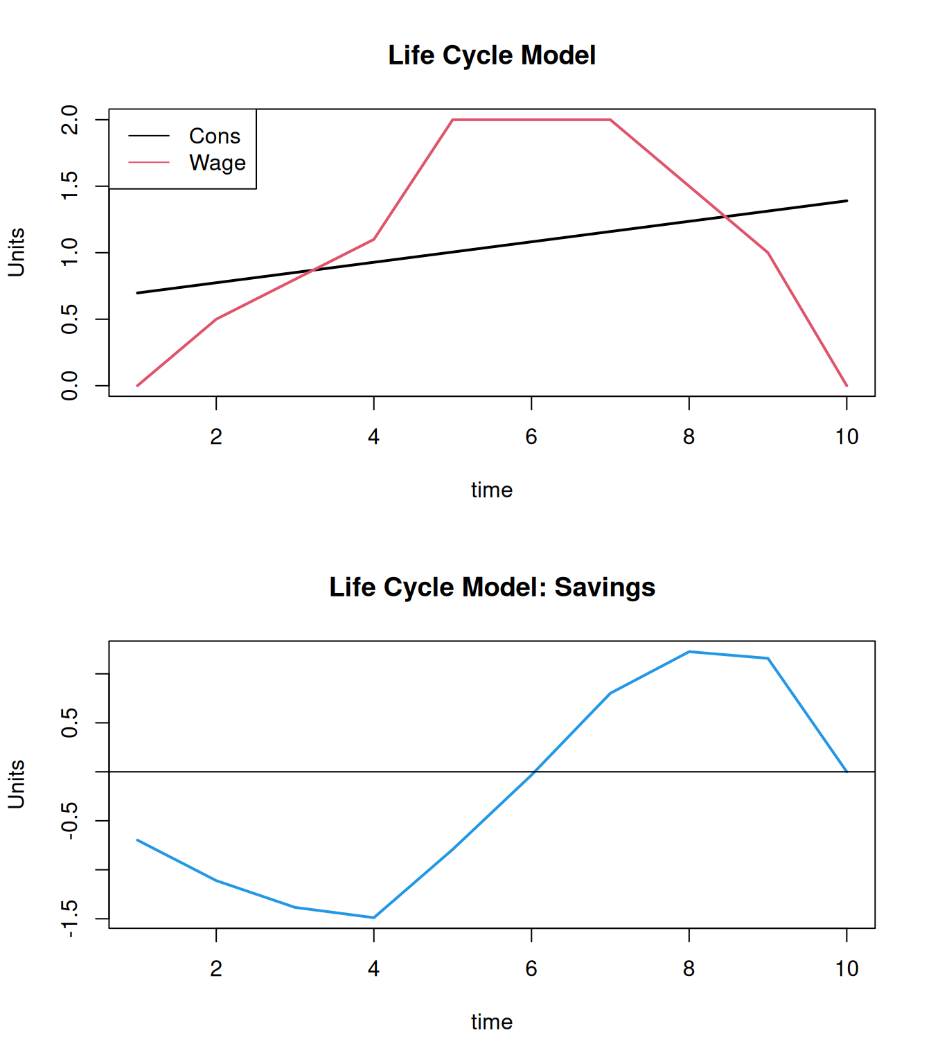
Consider an individual who lives n periods. At each period \(t\), he allocates his wage \(w_t\) between consumption \(c_t\) and saving \(S_t\). We suppose the interest rate \(r\) is constant. The individual’s problem is to maximize his future discounted utility: \[ \max_{S_t}\sum_{t=1}^T \beta^t u(S_{t-1}(1+r)+w_t-S_t), \] subject to \(S_0=S_T=0\). We therefore have to solve for \(S_t\), \(t=1,...,(T-1)\).
Consider the following case: \(u(c) = -exp(-c)\), \(\beta=0.9\), \(r=.0.2\), \(T=10\), and \(w=\{0,.5,.8,1.1,2,2,2,1.5,1,0\}\). The following graph shows the result:
Exercise 4.16 Write a function that solves the above dynamic optimization problem with \(r\in\{-.05,0.2,0.5\}\). Plot \(S_t\) and \(C_t\) for the different \(r_t\) and interpret your results.