Chapter 6 Numerical Calculus
6.1 Numerical Integration
We introduce the section with two examples. In the first, we consider the following portfolio optimization problem: \[\begin{equation} \max_{\omega_i} E\left[ U\left(\sum_{i=1}^n \omega_i Z_i\right)\right] \tag{6.1} \end{equation}\] subject to \[\begin{equation} \sum_{i=1}^n p_i(\omega_i-e_i)=0 \tag{6.2} \end{equation}\] It may look like a simple maximization problem, but it is not. The difficulty comes from the fact that we have to maximize an expected value, which can be written as: \[ E\left[ U\left(\sum_{i=1}^n \omega_i Z_i\right)\right] = \int\int\cdots\int U\left(\sum_{i=1}^n \omega_i Z_i\right) f(Z_1,Z_2,...,Z_n)dZ_1dZ_2\cdots dZ_n \] In the basic model, we assume that the preferences are mean-variance, an assumption that can be satisfied if either \(U()\) is quadratic or the vector \(Z\) is characterized by an elliptical distribution. In that case. only the mean and the variance matter, and the investors choose a combination of the risk free asset and the market portfolio. It simplifies the problem, but does not eliminate the need to compute integrals. For the applications bellow, we will assume that investors have a CRRA utility function \(u(c)=c^{1+\gamma}/(1+\gamma)\). For \(Z\), we will make different assumptions.
The second problem is quite simple. We only want to compute the future profit of a firm over the horizon \(t=[0,T]\), with \(q(t) = 3-(1+t+t^2)e^{-t}\), \(P(q(t)) = q(t)^{-2}\), and \(C(q(t)) = q(t)^{3/2}\). The profit is therefore is: \[\begin{equation} \int_0^T e^{-rt}[P(q(t))q(t) - C(q(t))]dt \tag{6.3} \end{equation}\] We will just cover few methods to understand the idea behind numerical integration, and conclude by showing you the tools available in R.
6.1.1 Newton-Cotes
The following graph shows the shape of the profit function in equation (6.3) for the horizon [0,4] with the Midpoint rule.
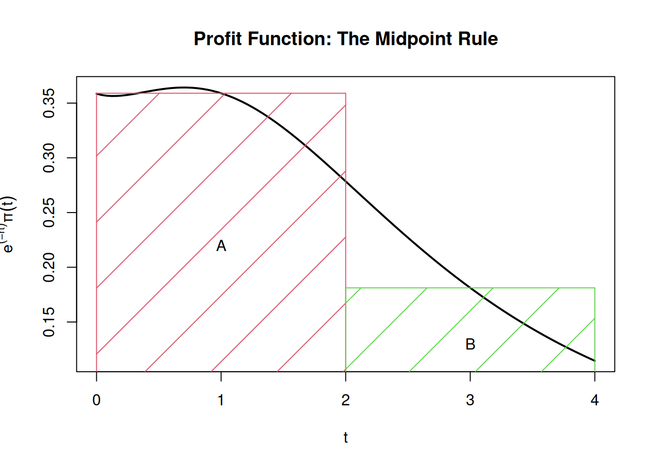
The midpoint rule approximate the integral by adding the areas of the rectangles A and B. The error of the method is given by \((b-a)^3f''(\xi)/96\), where \(\xi\) is between \(a\) and \(b\). Therefore, the method is exact when \(f(x)\) is a straight line because in that case \(f''(\xi)=0\). Here the integral as been divided in 2. In general, the method is: \[ \int_{a}^b f(x) dx \approx \sum_{i=1}^n hf(x_i) \] and the error is given by the expression \(h^2(b-a)f''(\xi)/24=(b-a)^3f(\xi)/(24n^2)\) for \(n\) equally spaced points, which implies that the error is of order \(n^{-2}\). In the example shown on the graph, \(n=2\), \(x_1=1\), \(x_2=3\), and \(h=2\). We can easily build a function for this method:
## [1] 1.058281The error is 2.8^{-5}. The Trapezoid rule is represented in the next graph.
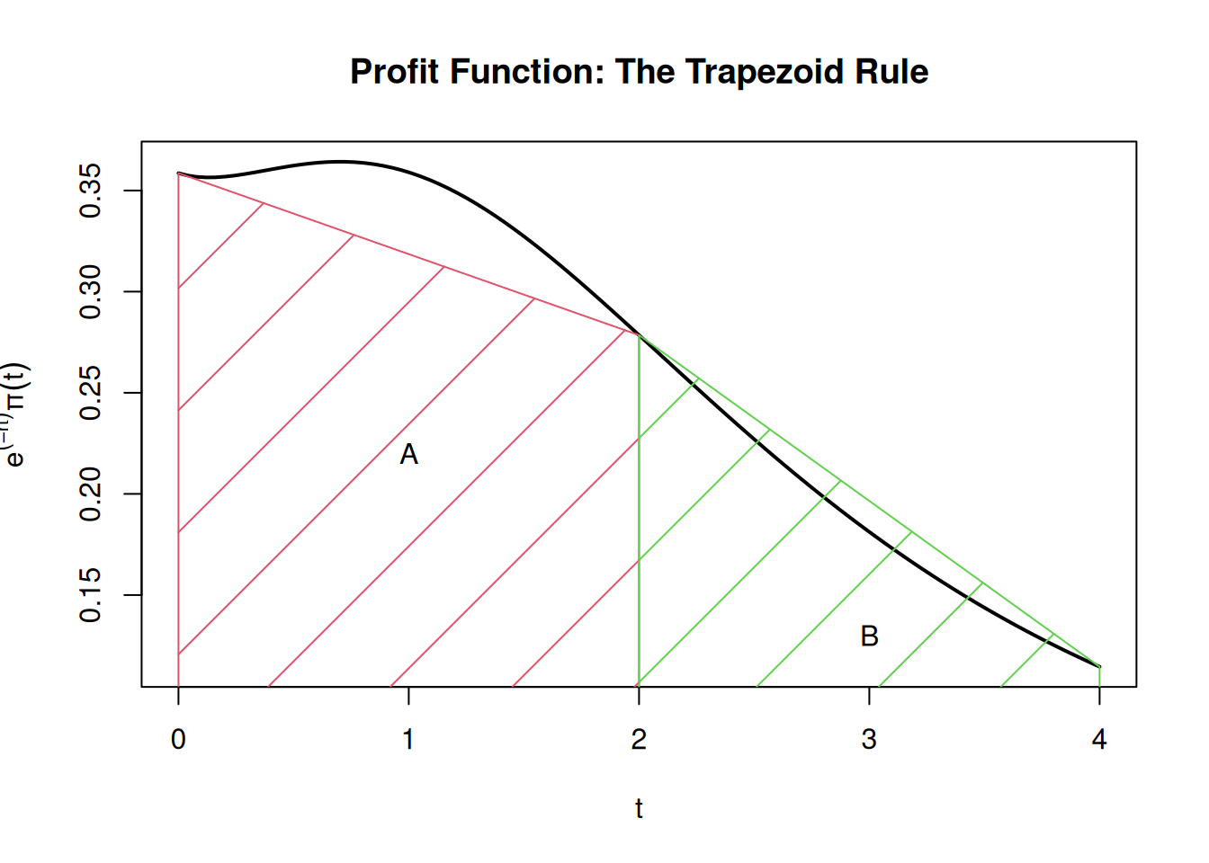
And the approximation is valid up to \(h^2(b-a)f''(\xi)/12\). Therefore, there is no clear difference between the two method. The method is \[ \int_{a}^b f(x) dx \approx \frac{h}{2}[f(a) + 2f(x_1) + \cdots + 2f(x_{n-1}) + f(b)] \]
Trapezoid <- function(f,a,b,n, ...)
{
    x <- seq(a,b,len=n)
    h <- x[2]-x[1]
    sum(h*c(f(x[-c(1,n)], ...),f(x[c(1,n)], ...)/2))
}
print(Int2 <- Trapezoid(Prof,0,4,20))
## [1] 1.058194The error is 6^{-5}, which a little higher than the one from the Midpoint rule. The Simpson’s Rule, approximate the function between points by a second order polynomial as shown on the following graph, and compute the true integral of this approximation.
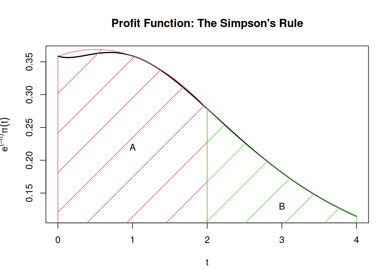
The error is of order \(n^{-4}\) (or \(O(h^4)\)) if the fourth derivative of \(f(x)\) is bounded. In fact, the expression for the error is \(h^4(b-a)f^{(4)}(\xi)/180\) which is the kind of expression used by functions such as integrate() in R to estimate the error. It can be computed as follows.
Simpson <- function(f,a,b,n, ...)
{
    n <- floor(n/2)*2+1
    x <- seq(a,b,len=n)
    z <- rep(c(4,2),(n-3)/2)
    z <- c(1,z,4,1)
    h <- x[2]-x[1]
    sum(z*f(x, ...)*h/3)
}
print(Int3 <- Simpson(Prof,0,4,20))
## [1] 1.058266The error is `r round(abs(Int3-Tint),6)’.
Suppose we want to compute \(E(X)\), where the density of \(X\) is \(f(x)\). Then, we need to get: \[ \int_{-\infty}^\infty xf(x)dx \] For the integral to be bounded, we need the integrand \(xf(x)\) to go to zero when \(|x|\) goes to infinity. Therefore, we can approximate the integral by \(\int_{a}^b xf(x)dx\), for some good choice of \(a\) and \(b\). Here, we allow the upper and lower bounds to be different. Let \(f(x)\) be the density of a \(N(5,1)\), here is few results using different \(a\) and \(b\):
## [1] 0.5512882## [1] 4.986499## [1] 4.999997It is clear here that \((-4,4)\) is not the right choice because the integrand is not centered at 0. In some special cases, we can recompute the same integral using a change of variables to make the bounds finite. For example, we can use the following change of variable for the above integral: \(x(z)=\log{[z/(1-z)]}\), which implies: \[ \int_{-\infty}^\infty xf(x)dx = \int_0^1 \frac{1}{z(1-z)}x(z)f(x(z))dz \] We can verify that the derivatives of the new integrand are all bounded if \(f(x)\) is the density of a normal distribution (a necessary requirement). The following, function would do the job:
f2 <- function(z)
{
    x <- log(z/(1-z))
    i <- ifelse(z==1 | z==0, 0, x*dnorm(x,mean=5)/(z*(1-z)))
    ifelse(abs(i)<1e-13,0,i)
}
Simpson(f2,0,1,40)
## [1] 0.896398The result is not very good. The problem here is that the function is close to zero almost everywhere except between 0.9 and 1, as we can see on the following graph:
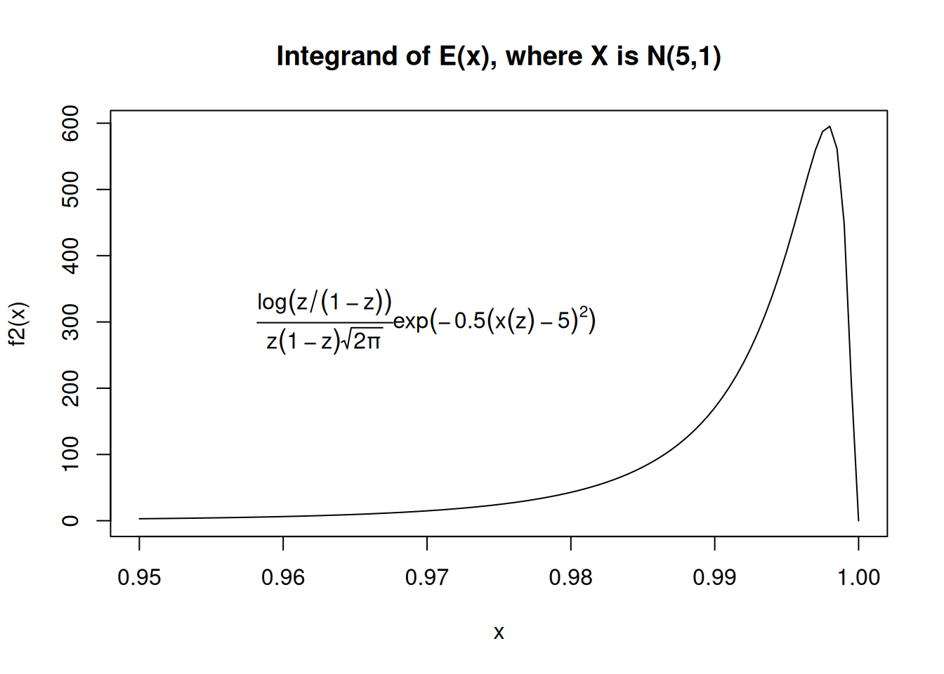
We need more points when the slope of the function changes quickly. We also want to avoid adding values that are dominated by rounding errors:
## [1] 4.9995956.1.2 Gauss Methods
The Gauss approach is to approximate the function using orthogonal basis, and to choose optimal weights and nodes simultaneously. In fact, the nodes and weights are such that \[ \int_a^b f(x)w(x)dx=\sum_{i=1}^n \omega_i f(x_i) \] holds exactly for all polynomial of degree \(2n-1\), \(f(x)\). The integrating function \(w(x)\) defines the inner product \(<f,g>\) so that the basis used to approximate \(f(x)\) are orthogonal and standardized with respect to this inner product (see Chapter 6 of Judd (1998) for more details). The different sets of basis are given in Table 6.3, page 204, of Judd (1998). There is an optimal quadrature for each \(w(x)\), but we can also do a change of variable when \(w(x)\) is missing. For example, the Gauss-Chebyshev, \(w(x)=(1-x^2)^{-1/2}\), and it is defined only between -1 and 1, but we can modify a simple integral as follows: \[ \int_a^b f(x)dx = \frac{b-a}{2} \int_{-1}^1 f\left(\frac{(x+1)(b-a)}{2}+a\right)\frac{(1-x^2)^{1/2}}{(1-x^2)^{1/2}}=\int_{-1}^1 g(x)(1-x^2)^{-1/2}dx \] which can be approximated as: \[ \begin{split} \int_{-1}^1 g(x)(1-x^2)^{-1/2}dx \approx & \frac{\pi}{n}\sum_{i=1}^n g(x_i)\\ = & \frac{\pi}{n}\sum_{i=1}^n \left(\frac{b-a}{2}f\left(\frac{(x_i+1)(b-a)}{2}+a\right)(1-x_i^2)^{1/2} \right) \end{split} \] with \[ x_i = \cos\left(\frac{2i-1}{2n}\pi\right) \] We see that the weights \(\omega_i\) for that method are all equal to \(\pi/n\). The following, implement the Gauss-Chebyshev method
GaussChebyshev <- function(f,a,b,n, ...)
{
    x <- cos((2*(1:n)-1)*pi/(2*n))
    y <- f((x+1)*(b-a)/2+a, ...)*(1-x^2)^(.5)*pi*(b-a)/(2*n)
    sum(y)
}
GaussChebyshev(f2,0,1,40)
## [1] 4.848546The function does not do as bad as the Simpson method which performs badly even with n=200:
## [1] 4.344921## [1] 4.999986The package statmod (Smyth and Chen (2026))has a tool to compute the nodes and weights for many quadratures. For example, we could rewrite the GaussChebyshev function as follows:
GaussChebyshev <- function(f,a,b,n, ...)
{
  x <- gauss.quad(n,kind="chebyshev1")$nodes
    y <- f((x+1)*(b-a)/2+a, ...)*(1-x^2)^(.5)*pi*(b-a)/(2*n)
  sum(y)
}
library(statmod)
GaussChebyshev(f2,0,1,200)
## [1] 4.999986For Gauss-Legendre, \(w(x)=1\), and the range is \([-1,1]\). It is therefore easy to compute \(\int_a^b f(x) dx\). We only need a change of variable for the range \([a,b]\). Here is the method:
GaussLegendre <- function(f,a,b,n, ...)
{
  res <- gauss.quad(n,kind="legendre")
  x <- res$nodes
  w <- res$weights
    y <- w*f((x+1)*(b-a)/2+a, ...)*(b-a)/2
    sum(y)
}
GaussLegendre(f2,0,1,200)
## [1] 4.999998The Gauss-Hermite quadrature is particularly useful to compute \(E(f(x))\) when \(x\sim N(\mu,\sigma^2)\). Indeed, its integrating function is \(w(x)=e^{-x^2}\), and the range is \([-\infty,\infty]\). The approximation is: \[ \int_{-\infty}^\infty f(y) e^{-y^2}dx \approx \sum_{i=1}^n \omega_i f(y_i) \] If we want to compute \(E[f(y)]\), where \(y\sim N(\mu,\sigma^2)\), we need to define the new variable \(x=(y-\mu)/(\sigma \sqrt{2})\) which implies: \[ E[f(y)] = \frac{1}{\sqrt{\pi}}\int_{-\infty}^\infty f(\sigma x\sqrt{2}+\mu)e^{-x^2} dx \] When we use the gauss.quad() function to generate the weights and nodes, \([a,b]\) is a function of the number of points \(n\). By increasing \(n\) we automatically increase \(a\) and \(|b|\), as we can see:
## [1] -1.6506801 -0.5246476 0.5246476 1.6506801## [1] -3.4361591 -2.5327317 -1.7566836 -1.0366108 -0.3429013 0.3429013
## [7] 1.0366108 1.7566836 2.5327317 3.4361591## [1] -5.3874809 -4.6036824 -3.9447640 -3.3478546 -2.7888061 -2.2549740
## [7] -1.7385377 -1.2340762 -0.7374737 -0.2453407 0.2453407 0.7374737
## [13] 1.2340762 1.7385377 2.2549740 2.7888061 3.3478546 3.9447640
## [19] 4.6036824 5.3874809Therefore, the function only depends on \(n\).
GaussHermite <- function(f,n, ...)
{
  res <- gauss.quad(n,kind="hermite")
  x <- res$nodes
  w <- res$weights
    y <- w*f(x, ...)
    sum(y)
}
Suppose we want to compute the expected utility \(E(u(c))\), where \(c=1+e^z\), \(z\equiv \log{(Z)} \sim N(\mu,\sigma^2)\) with, \(\mu=0.15\) and \(\sigma=0.25\), and \(u(c)=c^{1+\gamma}/(1+\gamma)\), with \(\gamma=-2\), then:
U <- function(x, mu, sigma, gamma)
{
    y <- sqrt(2)*sigma*x+mu
    c <- 1+exp(y)
    c^(1+gamma)/(1+gamma)/sqrt(pi)
}
GaussHermite(U,200,mu=.15,sigma=.25,gamma=-2)
## [1] -0.4631344We can then see the impact of increasing \(\sigma\) or \(\mu\)
## [1] -0.4646496## [1] -0.3792901The last quadrature is the Gauss-Laguerre. It is useful for computing future discounted profit or utility because \(w(x)=e^{-x}\). You can apply the quadrature in the next exercise.
Exercise 6.1 Use the Gauss-Laguerre quadrature to compute: \[ \eta\left(\frac{\eta-1}{\eta}\right)^{\eta-1}\int_0^{\infty} e^{-rt} m(t)^{1-\eta} dt , \] where \(m(t)=2-e^{-\lambda t}\), and \(\eta=0.8\). Try to reproduce Table 7.7, page 265 of Judd (1998) (you will need to do a change of variable here).
Exercise 6.2 Write a function that computes integrals with adaptive quadrature. The function starts with a small \(n\) and increases it until the value only changes by a certain tolerance level. Try to make it flexible and test it on the above examples.
6.1.3 Numerical integration with R
The function integrate can be use in general. However, we need to be careful. To estimate \(E(Y)\), where \(Y\sim N(5,1)\), we can do it as follows:
## 5 with absolute error < 6e-05It is not recommended to use big numbers instead of infinity as we can see:
## 0 with absolute error < 0The algorithm fails in that case. I recommend you to read carefully the help file for integrate before using it. The following shows how to compute the expected utility that we computed in the previous section.
U2 <- function(x, mu, sigma, gamma)
{
    c <- 1+exp(x)
    u <- c^(1+gamma)/(1+gamma)
    u*dnorm(x,mean=mu,sd=sigma)
}
f <- function(x)
    U2(x,.15,.25,-2)
integrate(f,-Inf,Inf)
## -0.4631344 with absolute error < 0.00011Exercise 6.3 In a statistical method called the Generalized Empirical Likelihood for a continuum, we need to compute an \(n\times n\) matrix \(C\) with \[ c_{ij}=\int_{-\infty}^\infty e^{-(x_i-x_j)^2t^2} \phi(t) dt, \] where \(\phi(t)\) is the density of the standardized normal distribution, and \(x_i\) is observation \(i\). Find a fast way to construct that matrix, and test your method with the \(2000\times 1\) vector \(x\) generated from a \(N(10,2)\).
6.2 Numerical derivatives with R {chap6-2}
Here is how to do numerical derivative in R. The following is taken from help(numericDeriv) file.
myenv <- new.env()
assign("mean", 0., envir = myenv)
assign("sd", 1., envir = myenv)
assign("x", c(-2,0,2), envir = myenv)
grad <- numericDeriv(quote(pnorm(x, mean, sd)), c("mean", "sd"), myenv)
attr(grad,"gradient")
## [,1] [,2]
## [1,] -0.05399097 0.1079819
## [2,] -0.39894228 0.0000000
## [3,] -0.05399097 -0.1079819Exercise 6.4 Write a function df(f,x) and ddf(f,x) that return the Jacobian and Hessian of \(f(x): \mathbb{R} ^n\rightarrow \mathbb{R} \), using numericDeriv.